While individual neurons have substantial computational power, neurons in populations can display actual intelligence. There is enormous computational power in populations of neurons, and even more when we can combine them in meaningful ways. In previous sections we looked at some of the behaviors that neurons in populations can accomplish, like precision extraction of a peak from a collection of imprecise samples, and the creation of brain waves from a collection of simple excitatory and inhibitory connections. Now we can consider population activity in the larger context of structured geometry. This includes layers, topography, and modular organization.

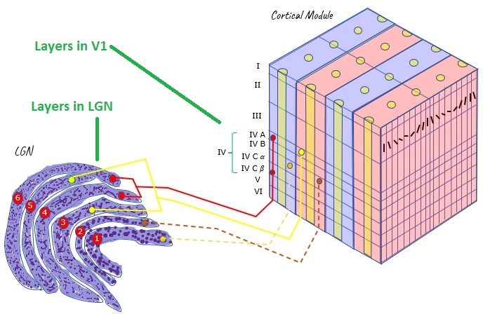
Layered Structures

There are many conveniently layered structures in the human brain. The figure shows the layering of the early visual pathway, from the thalamus to the cerebral cortex. Other layered structures in the brain include the hippocampus and the cerebellum, and we'll look at the retina and the brainstem in the next section. From such layered structures, we can often pick up electrical activity externally, because the currents tend to align.

Ions in neurons will tend to flow in the direction of electric fields. If there is a difference in potential between one part of a neuron and another, positively charged ions (sodium, potassium) will tend to migrate towards regions of negative potential, and vice versa. These flows create currents both inside and outside the cells, and these currents are what is measured when we place electrodes on the scalp for an EEG. Layered structures are very convenient because they tend to create measurable field potentials.

Scientists look for layered structures in the brain, because the currents line up. If all the currents are in different directions they will cancel out at long distances, and nothing will be measured on the scalp. However if they all line up then detectable scalp potentials are measurable, even though the signals diffuse considerably because of the conductive nature of brain tissue and the interference of the skull and meninges. Fortunately many of the important structures in the human brain are conveniently layered, including the cerebral and cerebellar cortex, the hippocampus, and sensorimotor structures like the retina and superior colliculus. The figure shows some typical patterns of current flow in layered brain structures.

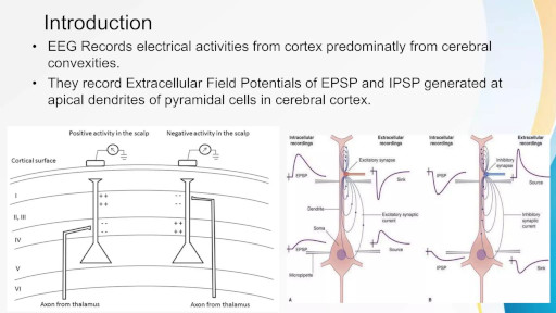
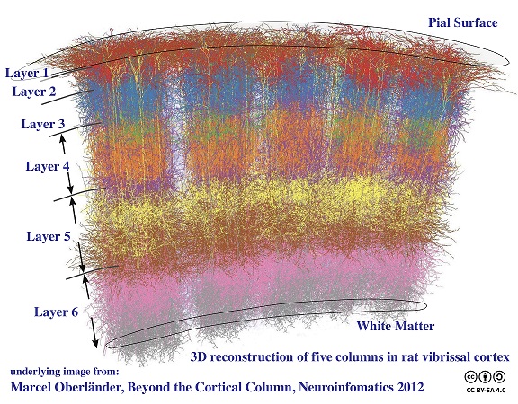
In the cerebral cortex, there are typically six identifiable layers (as shown in the figure), and there are large pyramidal neurons that are oriented vertically through the layers. The apical (vertical) dendrites from these neurons are aligned and generate large externally measurable currents. Within the cortex, such pyramidal cells cluster in layers 5 and 2/3, so the current measured externally is the sum of these activities.

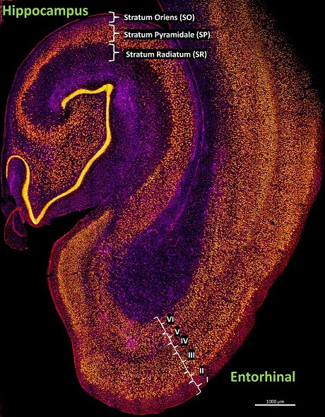
Here you can see a layered arrangement in the hippocampus, and its neighbor the entorhinal cortex. The hippocampus is considered allocortex and so has three layers, while the entorhinal cortex is neocortex and so has six layers.

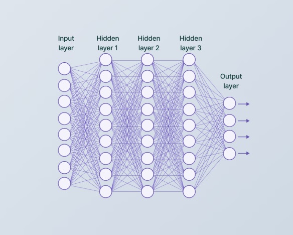
Topographic Organization

Sensorimotor wiring patters are often topographic, which means the topography of the environmental interface is maintained through the neural pathways. For example many visual areas are "retinotopic". Topography means that every point in the input space can be identified by its coordinates, and that the output space aligns with the input space and preserves the topography. The network below is not topographic, because everything is connected to everything else, and therefore the topography is lost between layers.

However the network below is topographic, because the coordinate system of the input space is maintained through the layers, until the very end.

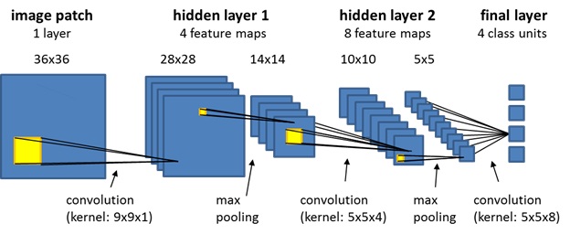
The network above is a "convolutional neural network" (CNN). The topographic mapping doesn't always have to be exactly point-to-point, it can be convolutional, which can entail point-to-region or region-to-point. Magnifications and distortions may also occur. For example the mapping of the retina into the primary visual cortex V1 is topographically tight but changes shape, from the smoothly curved retina it becomes approximately complex logarithmic in the cortex, the foveal area is magnified considerably relative to its size on the retina.

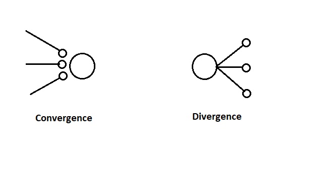
When specifying the topographic wiring, two of the key principles are the divergence and convergence of the connections, which determine the extent of any convolutional filtering. These are sometimes called "fan-out" and "fan-in" respectively, after the digital circuitry. These concepts are diagrammed below.

The convergence and divergence of neuronal projections can sometimes be adequately abstracted as "projection fields" from individual neurons. This intuition was suggested earlier in the sum-of-Gaussians model for retinal receptive fields. Sometimes such an abstraction can be computationally useful, especially when the time courses of the individual components are difficult to specify. On the other hand, the time courses matter, and so in more detailed models it becomes important to describe them individually.

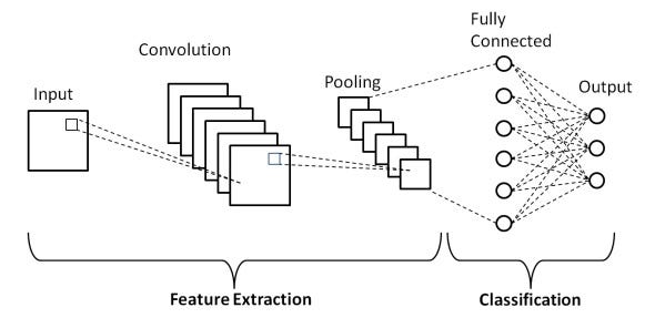
These concepts of convergence and divergence are vitally important when studying neural embeddings. We're almost ready to revisit this topic, but first we'll take a quick trip through a couple of example systems in the brain, to establish a comfort level and a model for additional study. But while we're on the topic, here is the overall architecture of a convolutional network from a machine learning standpoint. The left hand side of the diagram labeled "feature extraction" is where the progressively convergent convolutions occur, and the area on the right labeled "classification" is a different kind of network that gives us a one-hot code for the most likely object represented in the input. We'll talk more about machine learning later.

Modular Organization

In many brain areas the construction is "modular". This is true for example in just about the entire visual system. The modularity takes on different forms. In visual cortex V1, there are the well known orientation columns and ocular dominance columns, and also some color-related structures fondly known as "blobs" that become important in the connections to V2. While the modules may look a little different from one area to the next, the modular organization is ubiquitous in neural networks, across both brain areas and species. The figure shows an example of modularity in the visual cortex. The modularity takes different forms in different parts of the early visual system, from the honeycomb organization of rods and cones in the retina, to the relationship between narrow and wide field cells in the superior colliculus. Ensembles of neurons with simple connection motifs, are organized into larger interconnected modules in a network.

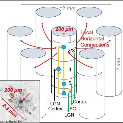
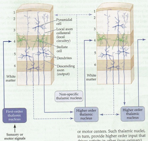
The concept of cerebral modularity goes back to Vernon Mountcastle in the early 70's, who proposed the organization of the neocortex into columns, minicolumns, and hypercolums, on the basis of both anatomy and electrophysiology. At that time, the work of Hubel and Wiesel had already been published, there were already existing examples of columnar organization. One of the first clues to the modular cortical organization is that incoming axons from the thalamus branch considerably more widely than many cortical neurons. Pyramidal dendrites may extend for several hundred microns, whereas incoming axons may branch over several millimeters.

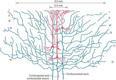
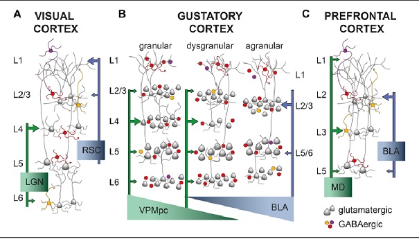
In spite of the complexity, a characteristic wiring pattern becomes clearly evident in the network. The neurons in different layers have distinct configurations. Those in deep layer 6 project back to the thalamus. The large pyramidal cells in layer 5 connect subcortically and serve as input to other cortical modules in layer 4 (along with inputs from the thalamus and other areas), whereas the smaller pyramidal cells in the upper layers 2/3 project to both the upper and lower pyramidal layers in other areas of cortex. There is a different emphasis on the neuron types and sizes in sensory vs motor areas and from one area of cortex to the next, but generally the motifs remain pretty consistent. This figure compares the somatosensory and primary motor cortex across the central sulcus.

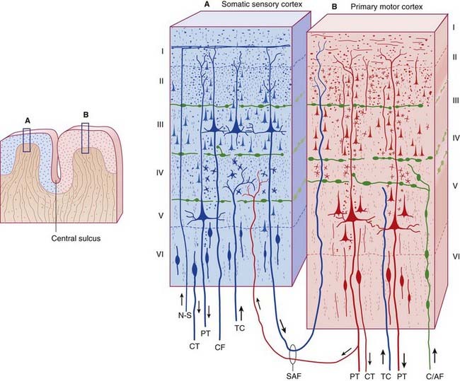
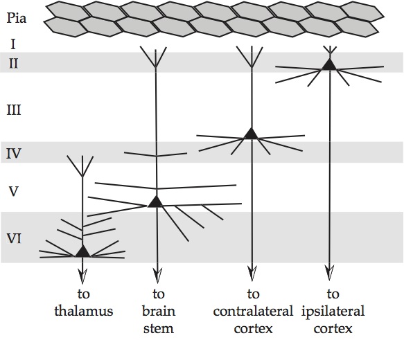
In the primary visual cortex the connection motif becomes very regular and very specific. Inputs from the thalamus arrive in layer 4, with the exception of a few koniocellular fibers from the LGN that target the blobs in the upper layers. The pyramidal cells in layer 5 project subcortically, to the basal ganglia, to the superior colliculus, and so on - whereas those in the upper layers project preferentially to other areas of visual cortex, both near and distant, and many send axons through the corpus callosum to connect with their counterparts in the contralateral hemisphere. The fusiform cells in layer 6 project back into the thalamus, so there is a loop from the thalamo-cortical relay cells going through layer 4 to these layer 6 neurons, and back to the thalamus.

Processing modules in the cortex can have varying sizes depending on their function. For example in the visual system (discussed in the next section), the "mini-columns" are very small, they're only about 60 microns wide and contain around 100 neurons. Whereas, a processing "column" is usually definable on the order of 500 microns, containing 50 to 100 mini-columns. Depending on the vocabulary used by an author, a "hypercolumn" is either equated with a column, or is a higher order collection of columns. In the visual system, a hypercolumn is considered a collection of columns, it's about 1-2 mm wide, which is much closer to the branching size of an incoming axon from the thalamus. The actual organization of a cortical area is shown in the figure, this particular one is from the rodent vibrissal cortex, which contains large easily accessible columns that have been modeled computationally.

Cerebral modularity is evident at many levels. It is usually most pronounced in the sensory areas, and less so in the frontal lobes and upper motor areas, although the lower motor areas are definitely topographic in many ways. It's still unclear how the different levels of architecture work together to perform computations and support brain waves. Many models exist, but they are mainly speculative, because the science is complex and the current state of technology doesn't always support it. As one moves centrally, the "receptive fields" of cortical neurons become more intricate, and it is sometimes difficult to know what to look for. For example the discovery of grid cells in the entorhinal cortex was made by pure chance (as was the discovery of motion-sensitive cortical neurons in the periphery of the visual field - there is a famous story of a tired scientist waving goodbye to her neurons after a failed experiment, only to have them start responding!), and now it turns out that the relationship between grid cells and place cells in the hippocampus is flexible - that relationship can be reprogrammed on the fly by bidirectional synapses in the hippocampus (Milstein et al 2021). Interestingly enough, the place cell maps seem to rotate in a coherent manner, which speaks to the compactification of the underlying network topology (Kinsky et al 2018)

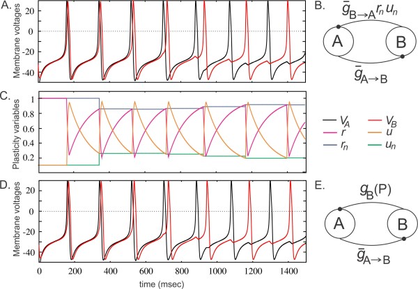
Cortical connectivity is flexible. The same basic architecture lends itself to multiple wiring patterns, in different regions of cortex. During development, the neurons position themselves in layers, and the connections are formed with a combination of genetic and environmental input. The genetic component determines (among other things) the types of plasticity available at synapses, while the data makes use of the plastic elements to configure the connection scheme and the resulting network behavior.

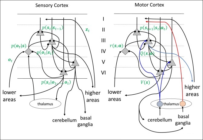
In many cases the circuitry can be tied directly to computational requirements. In the figure below, the symbols in green are related to predictive coding and Bayesian inference, which we'll discuss in an upcoming section.

Oscillatory Activity

Modular organization raises some interesting questions. For example, what exactly constitutes an oscillator? One can create an oscillator with a single neuron, or a pair of neurons, or a small population. What defines the boundaries of an oscillator, and why are oscillations sometimes brain-wide, to the point where they can be picked up all over the EEG?

Oscillatory activity is detectable in just about every central structure in the brain, and many of the peripheral structures too. Historically it has been rather arbitarily divided into alpha, beta, gamma, theta, and delta components on the basis of frequency, for example the theta rhythm is usually cited as being in the 5-8 Hz range, although it is more specific in particular brain structures (for example in humans the frontal midline theta associated with intense focal concentration comes in around 6.5 Hz, but even that varies). Given the very few neurons needed to generate an oscillator, it is somewhat surprising that large areas of the brain can sometimes be identified as oscillating in synchrony, and that large anatomical areas are sometimes dedicated to populations of oscillators (like the medial septal nucleus, which drives theta in the hippocampus).

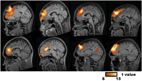
Generally speaking the population activity detectable on the scalp is an average of the neural activities inside the brain. There are other and sometimes more precise ways of looking at the generators of brain potentials and brain currents, for example the figure shows frontal midline theta generators detected with "synthetic aperture magnetometry" (Ishii et al 2014).

Oscillations occur at many different frequencies at once. One of the popular theories of brain function is the "dynamic assembly" theory, that posits cortical modules engage other modules with similar frequencies. The frequency content of a brain wave is frequently assessed through its power spectrum. There is considerable evidence of energy transfer between different frequencies in the power spectra of connected cerebral modules.

We looked at the Wilson-Cowan model because of its elementary behaviors in the phase plane, creating brain "waves" that can be triggered by inputs. In its original form, this model was simply a collection of omniconnected excitatory and inhibitory neurons, and depending on the synaptic weights one could see damped ringing in response to an input, or network-wide oscillations resembling brain waves. However a newer version of this model (Harris and Ermentrout, 2018) is topographic, and in the topographic version the oscillations don't have to involve the whole network (because it's not omni-connected, there is narrower convergence and divergence in the connection fields). In a connective topography like that found in the cerebral cortex, the oscillators can be narrow (just a few neurons) or wide (many neurons) depending on input and synaptic strength. They can create traveling waves as well as standing waves, with the appropriate boundary conditions. Furthermore, the region that comprises an oscillator can shrink or grow, depending on the local dynamics. An intense input at a particular location in the network can create a "hot spot" of dynamic activity, including oscillations at multiple frequencies that provide additional computational capability and endow the network with additional dynamic states.

This concept of "the boundary of an oscillator" is our introduction to "phase transitions". One can call the oscillating region a "phase" of activity, and here the usage is distinctly different from the angle associated with a sine wave. The usage here is more like "phase of matter", like ice-water-steam. When the network is in a down state, it's icy. When it's in an up state, it's liquid, and when it's oscillating and bursting it's steamy. The "phase of matter" of a patch of cortex has to do with how much energy is in it. At the boundary between a steamy place and a liquid place, is a "phase transition", an area which has very special properties. Strange and wonderful things occur in the phase transitions, they acquire special dynamics and special computational properties.

The delay associated with the refractory period is sometimes enough to trigger oscillations in a network, as shown by yet another variation of the Wilson-Cowan model (Meijer and Coombes, 2013). In general, introducing delays into either the synapses or the neurons themselves will alter the network's dynamic behavior, and modifying these delays even slightly is sometimes sufficient to create noticeable differences in population behavior. In many parts of the brain, even though neural behavior is stochastic, the time constants and transmission times are kept within narrow ranges, and often these are optimized through evolution to be "just right" for important computational functions. One such example is the gain adaptation in the retina, which has to work with topographic mapping in the superior colliculus while it's still developing (when an infant first opens its eyes, when it's receiving its first visual input). The point being, that plasticity has the capability to dramatically alter the dynamic behavior of neural networks, which in turn affects their computational abilities.

The purpose of the Wilson-Cowan model is to demonstrate network dynamics, and for this reason it is not inherently plastic. But it can be made that way, with some simple modifications to the synapses. However the resulting behavior is somewhat uninteresting as long as the network is omni-connected, the behavior is far more interesting in a 2d or 3d topographic context. When slightly modified, simple dynamic models can be combined with synaptic plasticity to yield intriguing behaviors, for example the figure below shows self-organized phase realignment of oscillators due to spike timing dependent plasticity (STDP) in a network of Morris-Lecar neurons.

An important form of self-organization occurs in networks of coupled oscillators. Such networks are described by the Kuramoto model and its extensions, and we'll look at that more carefully on the next page. Fundamentally Kuramoto describes the behavior of oscillators of the same frequency but at different phases, much akin to pendulums of the same length coupled by a mutual base (a rod, or string). The model has been solved exactly for bimodal frequency distributions, and characterized approximately for multimodal distributions. However it becomes mathematically challenging when one considers a continuous spectrum of frequencies, amplitudes, and phases. The resulting dynamics are high-dimensional, nonlinear, and difficult to visualize.

Another very important form of self-organized dynamics is self-organized criticality. We'll take a look at chaos and criticality in a moment, for now the heads-up is that there are dynamic systems that spontaneously evolve towards criticality. The study of this phenomenon is part of the larger consideration of how to program neural networks to adhere to certain kinds of desirable dynamics. Part of this has to do with designing filters at the single-neuron level, and part of it has to do with network wiring, and part of it has to do with adaptation and plasticity. Ultimately this issue relates to information geometry, which asks the question of how to best organize the data so it's both meaningful and computationally accessible. An understanding of the interaction between dynamics and information geometry is important. In a simple case it can be like a drum stick beating on a membrane, in a more complicated case (like a liquid state machine) it can become ripples on a pond. In this context it helps to understand things like holography and synthetic aperture radar (which, by the way, is what Norbert Wiener was working on when he came up with his theory of Brownian motion).

Population Models

Historically, the development of population models began with the Perceptron (Rosenblatt 1958). The Perceptron used a simple feed-forward architecture to accomplish linear separability. In the late 50's and early 60's, Bernard Widrow extended the Perceptron to multiple layer architectures, with Adaline and Madaline (Widrow 1962), and this led to the development and popularization of the least mean squares (LMS) adaptive algorithm by his student Ted Hoff (it's still called the Widrow-Hoff rule, or the Delta Rule). In the early 70's there was an explosion of network architectures relating to population dynamics, including models by Hugh Wilson and Jack Cowan, Stephen Grossberg, Shun-Ichi Amari, and others. In the mid-70's Kunihiko Fukushima created the first translation-invariant machine vision architecture, using multiple layers of feed-forward convolution networks (without any dynamics other than the presentation time of visual images). In the 80's people began trying to combine computational power with dynamics, and the results were spectacular and won Nobel prizes. The 80's saw the development of the Hopfield network, the Boltzmann machine, and many other powerful architectures that today are considered "foundational" for machine learning. There was also renewed interest in connectionism and topography, like McClelland and Rumelhart's classic text "Parallel Distributed Processing". The 90's saw the first large-scale computational modeling and engineering efforts for commercial purposes, and around the turn of the century neural networks were first identifed with "artificial intelligence". People like Sutton and Barto began to pay close attention to the various forms of learning, and their requirements in terms of neural networks. In the early 2000's various powerful neural network architectures appeared in the literature, like convolutional networks and recurrent networks, and there was the beginning of a concerted effort to understand learning rules, which led to the development of integrated GPU-friendly back-propagation for logistic regression and other computationally useful methods. Today, AI is commonplace, and there is a large commercial effort with many applications, because the technology is powerful. Transformers are everywhere. Neuroscience and machine learning have been informing each other ever since the very beginning, and unfortunately the human brain still remains a mystery because of the complexity, but mutual information continues and advances are being rapidly made on all fronts.

A population model in neuroscience, is something different from a complex machine learning architecture. Even though in some cases the basic concepts overlap, the neuroscience viewpoint is heavily focused on dynamics, and the ways in which neurons can move into and out of functional subpopulations. Machine learning engineers study this too, although in a different way (the two perspectives are beginning to merge). For example, one of the hot topics in neural networks is the dynamic assembly theory, and so far it's slow going because many of the modern machine learning tools don't handle dynamics very well. Part of the reason is, because dynamics require the numerical solution of differential equations, which in many cases is computationally more intensive than simple matrix multiplication. Population dynamics leads to the consideration of criticality in neural networks (Tian et al 2022, O'Byrne and Jerbi 2022), and indeed the human brain shows power-law scaling in much of its oscillatory behavior (Linkenkaer-Hanson et al 2001).

The behavior of individual neurons can significantly influence the behavior of neural populations. Examples abound in the hippocampus, where the first action potential generated by a CA3 neuron will travel antidromically (backwards) up the dendritic tree to influence both electrical activity and synaptic neurochemistry. In parallel with this behavior in the pyramidal neurons, nearby inhibitory interneurons will engage to suppress subsequent pyramidal spikes for some period of time, so that the "first" spike in the system is of great significance. Such behavior restricts machine models to spiking neurons, and it therefore requires that spiking dynamics be modeled by stochastic differential equations, because firing rate approximations aren't good enough.

Computationally, it's easier to look at a large number of neurons when they don't have to have specific architecture. There are "balance models" that take a similar approach to Wilson-Cowan, they just throw a bunch of neurons into a network with simple connectivity rules, and look at the range of useful dynamics and the nature of the resulting correlations. The idea of getting a neural network with specific topography to solve a large number of local differential equations in a small amount of time is challenging, even for the best simulator. There have been commercial applications using actual devices, neuromorphic FPGAs like Intel's Loihi and the Spinnaker chip, but these are generally small scale, involving less than 100,000 neurons. Approaches like the Neural Engineering Framework make it possible to create sophisticated behaviors with small numbers of neurons in these settings (populations of 50 to 100 neurons are sometimes) adquate to perform specific functions), but the gap between there and ChatGPT is enormous. Modern large language models contain literally billions of neurons, training them and running them continually requires a tremendous amount of power - however the results are self-evident. The interesting thing is, that none of the neural networks underlying modern AI, make use of population dynamics. They're not in the business of creating brain waves. In modern AI, dynamics would disrupt the computational process, it would clash with the back-propagation algorithms. However storing the entire history of the world in billions of neurons takes buildings full of GPUs, whereas our brains are only 15 cm long and we power ourselves with a sandwich.

State Transitions

According to the dynamic assembly theory, cerebral modules (which we tentatively and loosely equate with columnar organization) go in and out of functional and computational assemblies. What causes a group of neurons to engage with another group of neurons? This becomes a considerably complicated question in an environment full of oscillations with a myriad of different ways to synchronize them, couple and uncouple them, and regulate their presence or absence and their character.

With a bit of study, we become interested not only in the states the network can support, but also in the transitions between states and how they begin and end. Related to the dynamic assembly theory is another theory called the "critical brain theory", which posits that much of the brain operates near criticality, in other words near one or more phase transitions. These transitions would have to be carefully controlled, for dynamic assemblies to be useful in computations.

We'll review the concepts of state transitions and criticality extensively in the upcoming pages. For now we can note that there are dynamic local and global "states" in the network, and these states are both controlled by the brain and control the brain. We've already seen an example of network states in the Hopfield machine, which is a thermodynamic model in which the number of possible states can be conveniently calculated. We need to spend some more time talking about the Hopfield model, not just because it's the Nobel prize winning foundation for most of modern AI, but also because of its variations, which over the past 40 years include complex dynamic behaviors like coherent firing patterns, bursting oscillations, coexisting hidden attractors, multi-structure chaotic attractors, and network chimeras (Li et al 2024).

The basic idea of the Hopfield network is different from that of a traditional Perceptron-type network layer. A Hopfield network is an example of a "thermodynamic" model in that it relies on an energy function, which is repetitively minimized to find a final state. The network works by "gradient descent", like a ball rolling down an energy surface. As already mentioned, the secret to this network is that neural updates are asynchronous. Only one neuron at a time is allowed to be updated. Which neuron is chosen is important, network behaviors can be induced with particular selection algorithms. Generally the Monte Carlo method is used to ensure random selection (or selection from a desired distribution). Thermodynamic networks are very good at solving combinatorial optimization problems. The initial conditions are provided by the inputs, and the constraints are programmed into the synaptic matrix. The network simply runs until it finds an energy minimum. Sometimes it gets trapped in a local minimum, and in these cases a little bit of noise or a kick can cause it to resume its search, and there are also stochastic descent methods and other methods that work to avoid local minima. Some of these networks are guaranteed to converge to a global minimum (depending on the energy function and the connectivity), but some aren't, and in some cases the behavior can be adjusted by the judicious addition of additional neurons. The original Hopfield network stores "memories" (bit patterns), not very many, but the separability is good, although it is possible to confuse the network by engineering certain kinds of inputs. The more modern Hopfield network is very powerful, it functions as an hierarchical associative memory that can store a very large set of nearly continuous relationships. There are also so-called "autonomous" Hopfield networks, which find applications in systems that don't require real-time learning. They are interesting from a theoretical standpoint because they can be used to study the stochastic dynamics that lead to chaotic behaviors and critical network states.

Communication

The communication between neurons can be considerably different in various network states. The way a neuron responds to a synaptic input can be totally different when the population (or local dynamic) is in an up state or a down state. A single synapse can change its character depending on the postsynaptic membrane potential. These are highly complex and nonlinear relationships. Ultimately they are regulated by electrical and synaptic character of the neural environment (including specifically the glial environment).

There are certain kinds of neural network models (like some of the "graph neural networks", which we'll talk about shortly) that use a message-passing architecture rather than a straightforward set of synaptic connections. This means a large amount of information is being passed back and forth between neurons, more than just an analog value through a synapse. In a real brain the axes of transmission are related to the axes of encoding, and encoding is accomplished at the population level as well as the single-neuron level. In a recurrent architecture that tracks activity along a timeline, there is no need to pass large amounts of information between neurons, because the information is already present elsewhere. Neurons are perfectly capable of information routing, for example in the visual cortex the identity of an object is related to its position which in turn is related to its visual properties. If this collection of neurons has a common oscillation frequency in a dynamic assembly, then all a downstream system has to do is map that frequency, and in turn this will map all the information related to it. The frequency of oscillation will in effect "parameterize" the object and all its properties.

The volume and the efficiency of communication between neurons depends on their individual characteristics as well as their wiring into the network. And, synaptic properties can directly affect the ability to communicate, for example STP plasticity can make communication more efficient. There is extensive evidence that neural communication as well as information storage can be both more voluminous and more efficient in critical or nearly critical states. One reason is because more degrees of freedom are usually available near such states. Additionally, critical states usually entail long range coupling of the kind typically found between cerebral modules, and we'll review these concepts in considerable detail in the section on information theory.

Let's investigate the issue of criticality more closely. To begin with, we can look at chaotic behaviors. In the Hopfield network just discussed, chaos can be induced by simply adding self-recurrent connections. The reasons for chaos are many, and it has to be carefully controlled to make it computationally useful. What is interesting is that chaotic regions tend to cluster, much like oscillators. Chaotic systems tend to recruit each other, through their oscillatory behavior. There is useful computational behavior in the regions between clusters, which are often critical or super-critical in nature, have fractal geometric structure, and obey power law dynamics.