Two of the things engineers hate most are nonlinearities and random behavior. In a brain, the behavior is far from random, instead it is "stochastic" in that it has random elements while still possessing identifiable kernels. Stochastic behavior is often called "noise" when it's not wanted, but on the other hand sometimes it's wanted. For example a little noise can help a population of neurons escape a local energy minimum. We would like to be able to control noise in the same way that we control any other neural parameter, and in some cases this is possible, but generally it's not possible to get away from noise in a biological system. The best strategy is to get to know it and learn to make use of it. To further study neuronal and synaptic behavior, we would like to understand the sources of noise and the ways in which they can be controlled, and ultimately the ways in which stochasticity can be used to engineer specific network behaviors.
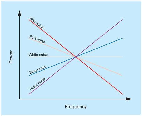
Types of NoiseWe can probe a system with noise, by treating it like a black box. However it matters what kind of noise we put into it. There is a special type of noise called "white noise" which has a flat frequency spectrum with no auto-correlation at any frequency. This is helpful because this kind of noise will "cancel itself out" in a linear system, and thus we can use it to expose nonlinearities. There are other types of noise, pink noise, red noise, blue noise... audio engineers know all about these and they're sometimes useful for neuroscientists too.
One of the characteristics of white noise is that its value at any given time does not depend on any of its previous values. This property uses a generator called a "Markov process", and in multiple dimensions this type of behavior results in a "random walk" like the Brownian motion studied by Norbert Wiener. If the system has memory however (like in a brain), the Markov property does not obtain, and neither are the kernels stationary. In this case we can use a set of lagged correlations to expose the influence of previous states. This is the approach taken in Volterra analysis.
Among the types of noise, two kinds that are especially important for neuroscientists are 1/f noise (also called "pink noise"), and 1/f 2 noise (also called red noise, or Brownian noise - not to be confused with brown noise which is something different). In white noise, the power spectrum is flat, every frequency has the same energy. In pink noise, the spectral density is inversely proportional to the frequency. 1/f noise is pink noise, it sounds like a waterfall. Red noise can be created by integrating white noise. In a leaky integrator such as that found in the peripheral oculomotor system, the red noise becomes Ornstein-Uhlenbeck noise, which is white below a threshold and red above.
Stochastic systems with memory are exceedingly complex to model. When they are stationary (which is almost never, in the brain), they can sometimes be decomposed into multiple discrete processes, however for the most part analyzing dynamic behavior in the phase plane requires performing repeated Monte Carlo experiments and plotting the results point by point. This effort is laborious and we only do it when we really have to. One of the practical problems is the generation of truly random numbers in volume. In the past this has been rate limited and sometimes requires special hardware, but recent advances in photonics have resulted in devices in the 3 gbps range, which will soon be commercially available. One of the successes of stochastic modeling has been the understanding of the chaotic trajectories that occur when we introduce recurrent positive feedback into a Hopfield network. Generally, positive feedback has to be carefully controlled in neural networks, otherwise the network goes into states resembling epilepsy, and it stops performing useful calculations.
Stochastic BehaviorNeurons are fundamentally stochastic. There is no deterministic timing like there often is in control systems. A neuron does not wait for the clock to tick. The brain achieves internal timing through membrane dynamics and local population dynamics, and ultimately population behavior is stochastic like the neurons. This should tell us that probability and statistics are useful ways of modeling and exploring the brain, and we have no choice but to study and understand the stochastic dynamics. For example the figure shows an approximation to the Hodgkin-Huxley dynamic using a stochastic leaky integrate-and-fire (Izhikevich) neuron. At some level this looks like a Hodgkin-Huxley dynamic, but what parts of it are essential? Does H-H introduce anything vitally different that we can't live without in our computational models?
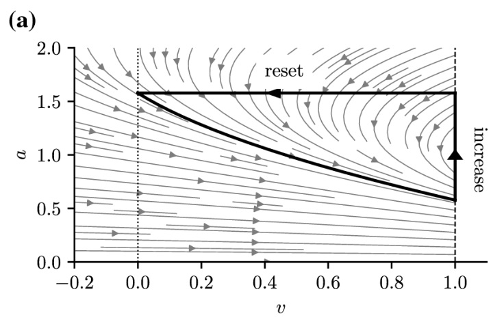
(figure from Holzhausen et al 2022)
Much can be learned from a single spike train from a neuron. If we have enough input, we can extract statistical information and visualize some of the underlying correlations and time constants. In single neurons and in populations, there are multiple operating modes that are overlaid on the stochastic behavior and the noisy input. These are modes in the traditional sense of differential equations, but they result from stochastic differential equations, which are often more difficult to solve and computationally more expensive. The prototypical stochastic process is Brownian motion, which can occur in one or more dimensions. It was extensively studied by Norbert Wiener, who published stochastic differential equations that describe it. (A brief perusal of the Ito calculus and the Malliavin calculus is recommended at this point, just to get the lay of the land).
Phase plane analysis is traditionally an engineering discipline, however it proves itself invaluable in brain biology. We need to be able to visualize the transitions between states, and the system trajectories. As a long time student of this discipline, I can recommend beginning with Shun-Ichi Amari's book Statistical Neurodynamics. Amari is also the godfather of information geometry, which we'll look at in detail later. If life is fair, Dr. Amari will be the next Nobel Prize winner.
In dynamics, we're interested in specific points in the phase plane called "bifurcations". These are points where the system behavior can take one of many paths. We saw an example in the Hodgkin-Huxley dynamics, where the bifurcation occurs at the point of threshold. Here the neuron can either relax back down to its resting potential, or generate an action potential by entering the limit cycle. In the Wilson-Cowan model referenced earlier, there is a similar threshold at which oscillations will begin to occur. If the input is below this threshold, the network exhibits an exponentially damped response and eventually returns to baseline. However if the input is above threshold, the network begins to oscillate and the trajectory in the phase plane enters a limit cycle. This behavior can be controlled by both the level of input and the synaptic weights. If the synaptic weights are weak, more input will be required to drive the network into oscillation. In a topographic network with limited lateral connectivity, oscillations may occur locally, and different parts of the topography may oscillate at different frequencies depending on the input and the local synaptic weights.
In a real brain, networks are multi-stable, meaning that the phase plane portrait can become quite complex. Phase plane analysis is an art as much as a science. Computers are helpful (Python has some wonderful libraries for visualizing dynamics), and ultimately neural network modeling is a cooperative effort between the computers and the researcher. To understand a network we have to go back and forth between the neuron models like Brian2 and the network models like PyTorch (and the integrations like PyNEST), varying parameters and seeing how to introduce new behaviors into the system and get rid of unwanted ones.
Chaotic BehaviorWhat is chaotic behavior? Chaos is defined as "extreme sensitivity to initial conditions". Without sophisticated mathematical and statistical tools, chaotic behavior is often mistaken for genuine randomness, but we can distinguish these conditions in several ways. One of the most important ways is visualization in the phase plane. If we can see the attractors, we can probably understand the trajectories too (and vice versa).
The word "chaos" implies wild and unorganized, and from a phenomenological standpoint, that is indeed the case. One way of looking at a chaotic signal is as an oscillator without a well defined frequency, phase, or amplitude. Such systems can be built electronically, they were explored by Leon Chua in his work at Hewlett-Packard (Chua 1994, Atan 2020). The circuit of a Chua oscillator is shown below. It uses a special component called a "Chua diode" that exhibits a negative resistance. But other than the diode and the inductance, it looks a lot like a nerve membrane (which is to say, a cable).

(figure by Chetvorno, CC0)
The dynamic (attractor) for this circuit is shown in the figure below. One can clearly see the trajectories in the phase plane. We are definitely interested in the areas circled in red, which are the areas where the trajectory leaves one limit cycle and enters another. Students of neuroscience will note the similarities between this phase plane portrait and that of a Hopfield network. We'll look at the various incarnations of Hopfield networks in a moment.
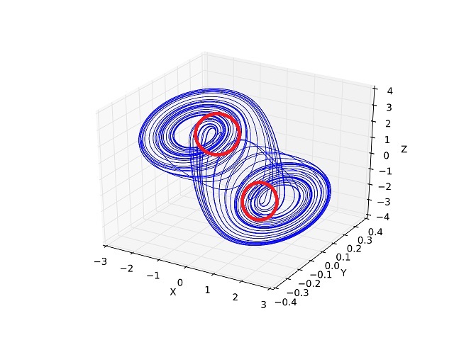
(figure by Shiyu Ji, CC BY-SA 4.0)
The shape of this attractor can be changed by altering the component values. Some of the available dynamics are shown in the next figure, along with the outputs (time series, spike trains) they generate. The negative resistance element can be replaced with an op-amp equivalent for modeling purposes, and a memristor can also be used (Atan 2020).
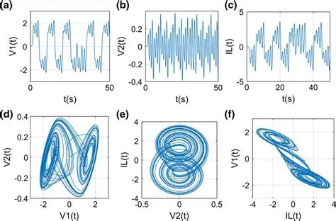
(figure from Atan 2020)
In the above dynamics, the critical points are the equilibrium points of the system. These are the points in phase space where the state variables stop changing over time. These points can be stable, unstable, or saddle points. They can be related to bifurcations, but they're not the same thing. Criticality does not equate with chaos (although many times, the two are found together and work together to generate the system dynamics).
Chaos In Neural NetworksThere are many neural network architectures that can result in chaotic behavior. Generally some form of positive feedback is involved, for example the Hopfield network can be made chaotic by simply adding self-recurrent synapses. Some of the possible architectures supporting chaotic behavior are shown below, many others are available.
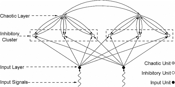
(figure from Zhu et al 2019)
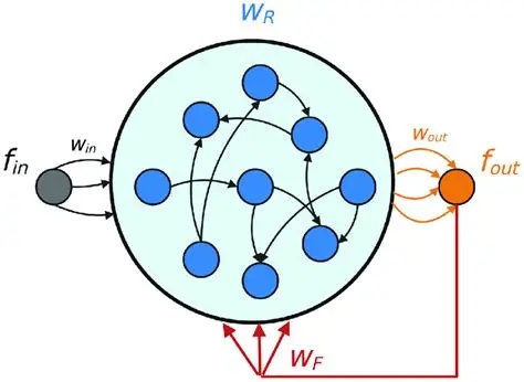
(figure from Liu L et al 2022)
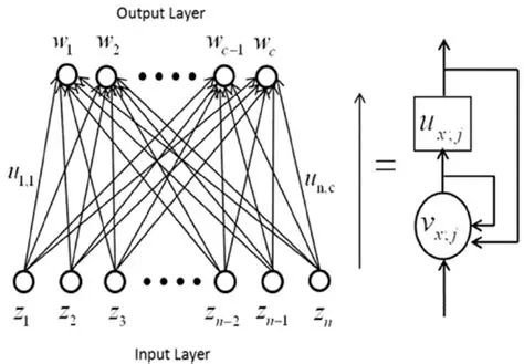
(figure from Qin et al 2014)
This last network looks very much like a neural integrator, and can be converted into one simply by adjusting the strength of U to reduce the chaos. We'll take a closer look at neural integrators in the section on oculomotor control.
Populations of neurons exhibiting chaotic behavior are often organized on the basis of "strange attractors" that may exhibit any manner of geometric catastrophes or oddball trajectories. Such an attractor is shown in the figure.
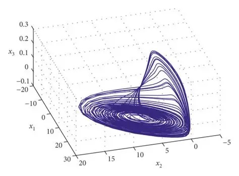
The above attractor is rather nicely behaved, though. These attractors get a lot weirder. Here is a chaotic attractor for the isolated delayed Hopfield network. Very strange, indeed.
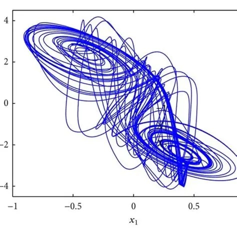
A "strange" chaotic attractor is characterized by its fractal structure. An attractor is called strange if it has a non-integer Hausdorff dimension. (A complete description of fractal geometry is beyond the scope of these pages, but plenty of information is available online with a simple Google search). Unlike normal attractors, strange attractors predict the formation of semi-stable patterns that lack a fixed spatial position and don't settle into fixed points. These become important when we begin to consider the thermodynamic ramifications of long range interactions (which is introduced below).
One of the important tools for understanding complex behavior in neural networks (and elucidating its relationship to fractal dynamics and chaotic attractors) is fractional calculus, first mentioned by Leibniz in 1695. Fractional calculus is an extension of ordinary calculus, it's an interesting and useful approach in both the discrete and continuous cases (He et al 2023), that lets us understand at least in part the effect of previous time frames on the moments. Fractional derivatives are not to be confused with fractal derivatives, which are something different.
Long Range InteractionsThe issue of long range interactions in coupled systems is closely related to nonlinear (and non-equilibrium) thermodynamics. Long range interactions are usually modeled by "coupling constants" that link modular subunits. for example there are chemical reactions in which each point in space is an oscillator. These are the reaction-diffusion systems studied by Ilya Prigogine, for which he was awarded the Nobel Prize in 1977. A well known example is the Belousov-Zhabotinsky reaction, shown below.
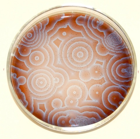
(image by Stephen Morris, Toronto Canada, CC BY 2.0)
(public domain image showing computer simulation of BZ reaction)
Long range interactions are often linked to fractal structures and particular kinds of power-function dynamics. In the chemical system shown above, which is fairly simple (malonic, citric, and sulfuric acids with some bromate, and cerium-4 sulfate, which is then reduced to cerium-3 by the reaction), the ratio of cerium-3 to cerium-4 oscillates, and sometimes these oscillations create spatial patterns, which can be wave-like and moving, and even stationary like standing waves.
The same principles apply in the brain. Long range interactions have been well studied with the Ising model. In these and similar cases, they lead to characteristic behaviors and geometries. Typically as the temperature of a magnet approaches the Curie temperature, the magnetic dipoles begin to lose their alignment and start to form chaotic clusters. These clusters in turn, may couple over long distances and induce geometry in the system as a whole. Groups of clusters may also form "dynamic assemblies" that communicate with each other but not with other clusters. In common, at the boundary between neighboring clusters, is a chaotic region that is typically fractal in nature and exhibits power-law dynamics.
Long range interactions are also implicitly included in the "coupling constants" of the Kuramoto model. In the BZ simulation above, the oscillators are mapped into a "tensor field" over space, so that each point has an amplitude, frequency, and phase. The coupling constants are necessarily vague, if they were described explicitly they would amount to an infinite dimensional matrix. They are useful for computation but their specific relationship with physical and network properties is sometimes poorly defined. This study becomes even more difficult in the high dimensional spaces typically associated with Bayesian information processing.
Information TheoryWhat does chaos have to do with stochastic behavior? Do neurons still communicate in chaotic states? Yes, they do! In fact sometimes, more information can be passed more quickly and more reliably, when the network is in a chaotic state. This may seem counter-intuitive at first, but we can look at an example of how this happens, by taking a quick detour into information theory. To understand information in neural networks, we need two key concepts: the Fisher information, and the Kullback-Leibler divergence. Both of these derive from an information-theoretic approach to entropy.
Information theory is only interested in "new" information. If it's old information, it's not really information (because you already have it). Information theory looks at the degrees of freedom in a data set. We can use the example of a coin flip to illustrate the principle. There are only two possible outcomes, let's say tails is 0 and heads is 1. But you don't know in advance that there are only two states, you have to discover this - so you start performing experiments and looking at outcomes. After a while, you begin to see that the result is always 0 or 1, it's never 2 or 5. So whenever you get a 0 or a 1, you're not really getting any new information about the system, you're only getting the "state at a particular time". But now let's say you suddenly get a 5. This is new information, it's never happened before. It it... "surprising". And because of this, you have to update your two-state model, because now you know there's a third state.
Information theory requires knowledge of the underlying probability distributions. This is because information is defined in terms of entropy. The Shannon entropy in binary terms (for a bit stream) is defined as
S = - Σ p log2(p)
where p is the probability associated with a bit. In a continuous setting this becomes the von Neumann entropy. How do you get probability distributions? Generally, you have to estimate them. That's what Bayesian inference is for, and why it's so important in neural networks. The estimate of a probability distribution is akin to a "belief", because the brain doesn't wait around for an infinite number of frequentist trials before making judgements about the underlying generators. Instead, it updates its beliefs on-the-fly, by updating the probability distributions based on new incoming information. In a timeline architecture, each new data point can cause a re-evaluation of all the probabilities between events, and this is one reason we're interested in micro-causality in real time.
This concept is worth restating in a different way. Sometimes, network states can be directly related to probability distributions. There are two basic approaches to probability, the frequentist approach and the Bayesian approach. In the frequentist approach, the probability of an event is its asymptotic occurrence after an infinite number of trials. Using this approach, we have to flip the coin an infinite number of times before reaching the conclusion that the probability of heads is 1/2. However the Bayesian approach is about "belief", and one's belief could be very different from the ground truth. In the Bayesian approach, every time you get a new piece of data, you update your belief. Gradually over time, your belief comes to align with the real probability - however you don't need an infinite number of trials to accomplish this, generally you only need a few examples before your belief stops changing. In the Bayesian approach, you use a model of the generator, and you're altering the model parameters every time you update your belief. In a neural network, model parameters are generally associated with "hidden neurons" or "hidden layers", that don't receive direct sensory input but instead receive their inputs from other internal neurons. This way, the hidden neurons come to model the statistics of combinations of inputs. This is the basis for the combinatorial optimization that we saw in the Hopfield network.
The interpretation of information in information theory is something along the lines of "surprise", and the human brain has some peculiar behaviors when it's surprised (when it either gets new information, or when it's missing information). There is an event related potential called the P300 that occurs in portions of the dorsal attention system when one gets surprised (a good way to elicit a P300 is with nonsensical information, like "I take my coffee with cream and dog"). The P300 has two components, an early component that "notices" the condition, and a later component that acts on it. The P300b is sometimes associated with a classic "startle" reaction in humans, which is characteristic and usually involves head and eye movements.
Information GeometryMany machine learning techniques are designed for the specific purpose of visualization. For example there are clustering algorithms that change the coordinate axes in such a way that similar points appear closer together, and this way groupings within the data can be more easily visualized. As with any kind of curve fitting, this is a model based approach and one must be careful to discover the appropriate number of useful parameters with which to describe the system. If a receptor binding curve has two components you don't want to fit a four-component model to it, so one has to work with the data to discover an appropriate model.
Information geometry handles the application of probabilistic methods to non-Euclidean coordinate systems. These non-Cartesian coordinates can arise in a number of ways, like when distributions or data sets are skewed, or when the underlying generators are nonlinear, or when the coordinate axes are rearranged, or when we simply want to look at things in a different way. The information geometric method works by mapping the (modified) data onto a Riemann surface (a "manifold"), and using the Fisher information as a metric on this surface. In this way the distance between distributions becomes directly related to the Kullback-Leibler divergence. What do these terms mean?
The Fisher information is a way of measuring the amount of information an observable random variable X carries about an unknown parameter θ of a distribution that models X. If you're not familiar with Bayesian inference I can highly recommend taking a time out to learn the basics. It's the foundation for much of modern AI, not to mention its myriad applications in neuroscience. An excellent set of introductions can be found on YouTube and at Coursera.
The Kullback-Leibler divergence measures how much one probability distribution differs from another. Restated in a different way, it quantifies the extra information cost incurred when using one distribution to approximate another. The K-L divergence is also called "relative entropy". Mathematically, if P and Q are two distributions,
DKL (P || Q) = Σx P(x) log (P(x) / Q(x))
Information geometry can be useful for determining the structure of "latent spaces", which are the hidden layers containing the model parameters in the network. In diffusion models the phase transitions in the latent space acquire a fractal structure, characterized by abrupt changes in the Fisher metric (Lobashev et al 2025). The "nearness" of points in a representation space can sometimes be visualized with PCA (in the linear or nearly linear case) or t-SNE (a form of nearest-neighbor analysis) in the nonlinear case, but the ultimate toolset for visualization is information geometry. Visualizing the organization of information in a synaptic matrix is one of the many important applications of information geometry.
An excellent introduction to information geometry is the review by Nielsen (2020). Some knowledge of differential geometry is needed to understand it. For that, I can recommend the excellent videos by user "eigenchris" on YouTube, entitled "Tensors for Beginners" and "Tensor Calculus". The tensor notation is very helpful in the machine learning literature and should be studied. Take your time, it took me about 3 months to become comfortable with it. The relationships between the dot products and the metric tensors are of crucial importance, as they relate directly to the calculations that must be performed, both in the GPU and in neural networks.
The figure shows some of the territory covered by information geometry.
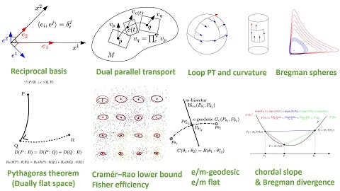
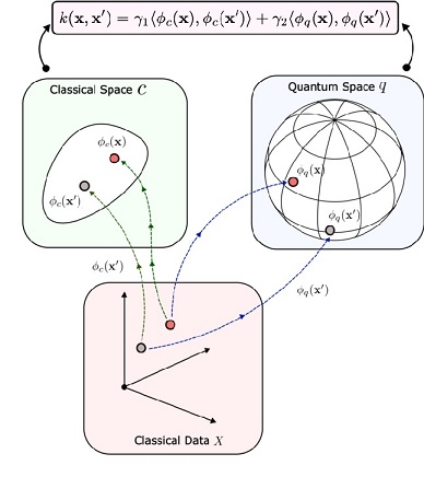
The next figure shows an advanced but intuitive application of information geometry. We'll talk about quantum computing, some exposure to it is important as there are presently many neuromorphic quantum devices in development.
Information Transmission In Critical StatesHow is it that information can sometimes be transmitted more reliably when everything in the system is in a chaotic and near-critical state? Part of the answer lies in the degrees of freedom available around critical states. Generally, there are more degrees of freedom near bifurcation points, because once the system is on a trajectory it tends to stay there, whereas at a bifurcation point there is a choice among many trajectories. Generally in neurons and neural populations, a bifurcation point is associated with a change in state. The neuron or population may begin oscillating, or bursting. In such situations, the information is encoded in a different way. For example in bursting neurons in the oculomotor system, the target location is indicated by the peak of burst rate within a population, whereas the velocity of the eye movement is encoded into the burst rate at the selected target position. This arrangement allows the afferent systems to communicate with the targeting system in a consistent manner, and it allows the targeting system to make an easy and logical decision when the input systems provide more than one target.
Armed with this overview of populations of neurons, let's take a look at some real systems. We'll choose a sensory system and a motor system. The visual and oculomotor systems are excellent candidates because they've been well studied and they're exemplary of many useful architectures and functions. After reviewing these systems, we'll have one example each of networks that operate at T << 0 and T >> 0 respectively, along the neural timeline. These networks meet for example, when the organism needs to track a moving target. Usually a saccade acquires the target, and then smooth pursuit follows until such time as ocular drift or pursuit error exceeds a threshold, at which point a small saccade corrects the error and pursuit resumes. When the prey stops, the eye movements stop too, the fixation (omnipause) neurons become active, and gaze is fixed on the target, with a few continuing microtremors to ensure the retina doesn't over-adapt to the static image.
We'll look at the visual and oculomotor systems as examples of brain networks that live on opposite sides of T=0. If you already know about these systems and you're primarily interested in computational modeling, you can skip directly to the modeling pages.
Next: The Visual System |