In a finite element model, each tiny little piece of a mesh becomes a computational compartment. If we have a triangular mesh representing a surface, it's a membrane and we're looking at the flow of ions (and other molecules) across the membrane. If it's a tetrahedral or hexahedral mesh the elements represent volumes, and we can look at flows into and out of tiny little volumes in the cell. If we're being ambitious, we can mesh the outside of the cell too - that is to say, the space between the cell and surface of our volume conduction sphere. Here the specter of scale raises its scary little head again, and I'll let you do the math on how many 25 nm cubes will fit into a 1500 cm³ brain. For this reason finite element modeling is usually done on very small patches of membrane, or very small volumes of a cell. A single leaflet or small branch of an astrocyte would be a good candidate for finite element modeling. FEM excels with real geometry, it accounts for all the nooks and crannies of a real membrane, whereas the traditional cable model still treats all the compartments as cylinders.

It's time to consider the finite element model in a larger context. In today's world, data sets with billions of points are not uncommon, and the reality is we can quickly and easily fit the whole array into a GPU. At the point where we actually start doing calculations, the finite elements are inextricably bound to the geometry, so it makes total sense to keep the two together. When done this way, the physical variables become pieces of data attached to the elements of the mesh. For example if we were to consider a temperature field across our geometry, the temperature at any given point on the mesh would be a number attached to a vertex. In a way this is very reminiscent of the Kirchoff law in a cable model, but in this case we're doing "multi"-physics, so it's not just the currents we care about, it's the fluid flows and mechanical forces too. Why do we care about fluid flows and mechanical forces? The one-word answer is: calcium. Calcium responds to external electromagnetic fields, and it affects the cytoskeleton. It is the perfect messenger between the field and the geometry.

The mesh contains two distinct pieces of information: the geometry, and the topology. The geometry is the coordinates of the points in space, the topology is the way they're connected. On a lattice each vertex is connected to its nearest neighbors. In a multi dimensional topology this may not be the case, we may have extensive sets of distant connections. The simplest way to conceive a volumetric mesh is as a set of voxels. Voxels are like pixels, except in 3 dimensions. They're like little volume elements, and when they all have the same size it makes computation very convenient. In terms of the geometry, the coordinates define for us some axes, call them x y and z. We have faces along each axis, and the physics wants us to determine the flow through each face and the circulation along the boundary of each face. In the case of charge, our flows are ions. In the case of the fluid dynamics, they're molecules of all kinds, not just ions. In the case of mechanical forces, our flows are the forces themselves, the differentials on the boundaries of the cells. Using these principles we can calculate the physics on each mesh element, deriving our answers using mathematical principles like Stokes' theorem and Green's theorem.

So there is a substantial amount of calculation, but the good news is that certain kinds of meshes make this easy. We can use the methods of discrete exterior calculus to approximate everything we need. How that works is, we use volume elements to measure other volume elements. DEC depends on our ability to calculate "duals", which are a bit like orthogonal complements. Once we have the dual, an integral gets translated into a set of much simpler operations (like, we add up the values at all the nearest neighbors of a point), and a derivative becomes a simple subtraction. Done this way, we can create a large but symmetric matrix representing a linear mapping f = M u, where u are the nodal values and our matrix M can be broken down into multiple parts when necessary. These are examples of the types of meshes DEC excels at:

     

     

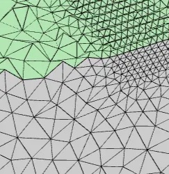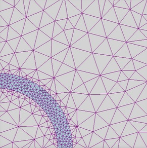
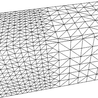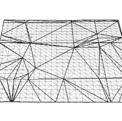
As you can see, the faces don't have to be regular, and they don't have to be perfect. However a well behaved mesh makes computation a lot easier, and to get a well behaved mesh from an arbitrary starting point, we need a mesh tool that lets us refine the quality of the mesh. This tool has to be able to handle billions of vertices, which automatically eliminates 90% of the meshing "ecosystem". Most mesh tools will crash instantly if you try to load that many nodes, and the ones that don't usually cost money. If you need to do this yourself because you have special scientific needs, I can save you some trouble because I've been all over this space. (Even in the last 30 days!) You'll need to find the specific parts of each public domain package that actually work. For instance open3d's sampling works great, but the export of OBJ files is funky, it leaves extra fields after the vertex coordinates and things like that. On the other hand, tetgen requires a perfect manifold mesh, so you have to clean and repair your mesh up front, and pymeshfix works pretty well for that singular purpose but trimesh crashes with big meshes. Even VTK crashes with big meshes - even after being field tested in the National Labs for 20 years. If you're having difficulty finding tools that work, please visit my sister site neural-modeling.org.

A face on a mesh is not a "finite element". A finite element is a function. This function is made up of a linear combination of basis elements, which are also functions. The simplest way to understand this is to look at the case of linear interpolation. In this case, our functions are straight lines, having the value 1 at exactly one vertex, and 0 at every other vertex. Such a set of basis functions looks like this:



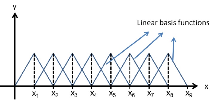
These functions are "piece-wise linear". In three dimensions they might look like this:



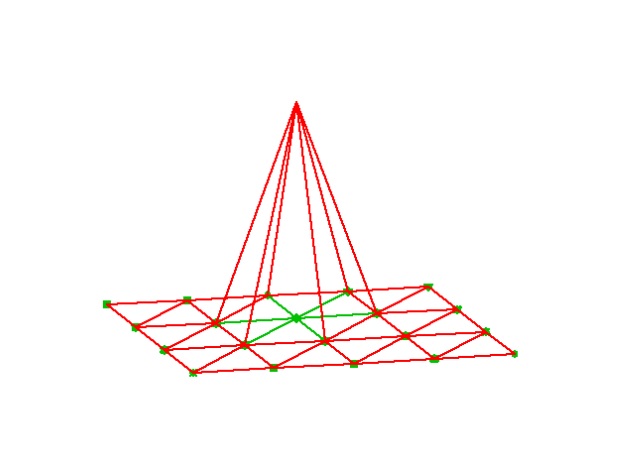
We estimate the values at the centers of faces by interpolating along edge elements. As mentioned, these elements already contain all the information we need to make the calculations. When we do things this way, a neuron doesn't have just one membrane potential, it has many. It has one at every vertex, or every face. Because of the physical continuity constraints we impose on the solver, these membrane potentials will be approximately as smooth as the mesh surface is, and since the mesh surface is manifold we are guaranteed piece-wise continuity.

The computations are performed on vertices and their neighbors, meaning the simulator has to know about the topology. It has to keep the list of which vertices belong to which faces, and what their orientations are. The easiest way to accomplish this is to download the entire mesh into the GPU. nVidia has a nice physics library called Warp that's friendly to both Python and C++ and has built-in tools for mesh calculations. The one caveat is the GPU will only perform 64-bit math, if you want more than that you have to use an emulator like Sleef (or write one). Besides the mesh, the other thing you'll need is a set of algorithms to execute the operations you actually want to perform on the mesh, which you'll have to download into the GPU along with the mesh data. The GPU becomes the simulator, it simply runs down the list of mesh elements and applies each algorithm in order, and once it's done with a round of computations you can upload the results back into the CPU or simply display them straight from the GPU.

Even nVidia's older GPU's are exceedingly fast. An old GTX-1080 still has 11 gB of memory and a compute rating of 6, which means you can use it with Warp and mesh sizes up to about half a billion points. The newer RTX-5090 is super-powerful, it uses a Blackwell class engine which is the same thing they put into an H100. It has a compute rating of 12, exactly the same as an H100. You can put two of these into a PC and you'll have an unrivaled personal simulation engine. It won't be as fast as 100,000 Docker containers in the cloud, but it'll be very darn fast. You'll be able to run molecular dynamics simulations on it (I know because I'm doing it!).

On meshes of the kind shown in the diagrams, Maxwell's equations take on a very simple form. Instead of four complicated equations:



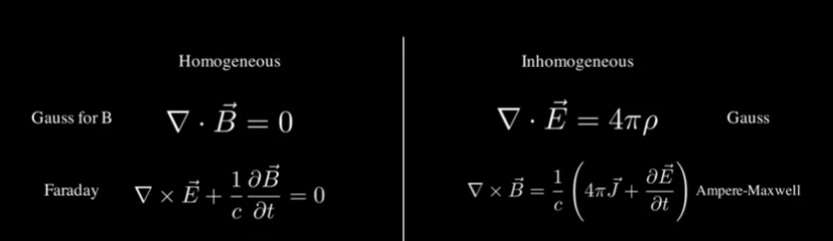
the meshes in combination with the methods of discrete exterior calculus give us two simple ones:



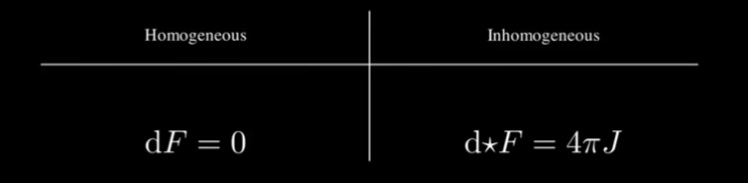
The '_*' operator in the last equation is the Hodge star, which we calculate on each element of a mesh. Done this way, Maxwell's equations reduce to trips around mesh boundaries.

This video clarifies the basics of discrete exterior calculus in 25 minutes. For a slower and broader perspective, there is the excellent series by Keenan Crane.

The result of a finite element simulation is a function on a mesh. In many cases it's a scalar function, like a heat map of local temperature. In other cases it may be a vector field, like the velocities of charged particles from one mesh element to the next. The finite element method solves partial differential equations on a geometry, and in most cases the first need is to save the information, and the second is to visualize it. The per-tick output of a finite element solution is enormous, if you have a million vertices your per-tick files might be 100 mB each. There is currently no standard for exchanging neuroscientific simulation results. It's hard to get the per-tick output into a public format. The common denominator is the CSV file, which loads into Pandas with a single command. Once your data is in Pandas, you can do anything with it, slice and dice it, reshape it, edit it as you wish. (Pandas is a lot like R, it's a data science language that works with data frames, it's very powerful and more Python-friendly than R).

Finite elements can access things that are too small for compartments. For example, let's talk about dendritic spines. These are tiny little protrusions from the surface of a dendritic shaft. They are "filopodia", they have very thin stalks with a small head at the tip, and the head can have varying shape and volume from point-like endings to mushroom shaped caps. Spines don't really "have" morphology, they're constantly moving and changing. The only thing that keeps them stable is their attachments to synapses and astrocytes. They grow, they shrink, they change along with the signals flowing through them. Dendritic spines carry synapses on their heads. These synapses are wrapped by astrocytes, on both sides. They have a life cycle, they're born, they mature and then change size and shape with plasticity, and eventually they're subject to pruning and get removed when they're no longer useful. If we'd like to know what happens in the stalk of a dendritic spine (which is valuable information for many reasons), we can try using a cable model (many people have), in which case we'll see the obvious. Stalks are tiny so they typically have a high electrical impedance because ion flow through a 50 nm space is difficult. Inside a stalk are actin filaments that take up a considerable portion of the 50 nm radius. The actin is involved in the transport of other molecules, from ER saccules at the base of the stalk to the tip of the synapse.

One of the reasons stalks are important, is a concept called "glutamate spillover". The idea is that in an excitatory synapse, a considerable amount of glutamate is released with each action potential. The neurotransmitter then diffuses across the cleft, and diffuses out of the cleft, where it's sucked up by astrocytes through EAAT transporters. However when there's a lot of activity, there's so much glutamate that it spills over out of the synaptic area and down the shaft of the dendritic spine. Here along the shaft of the spine, there are additional glutamate receptors, so the spine shaft "detects" this condition, and then it can adjust itself according to the amount of spillover. If there are receptors along the stalk they'll likely involve ion channels too, and that is in fact the case. So a spillover event will influence the subsequent activity of the postsynaptic side of the synapse, which is another aspect of plasticity that's a little different from the usual LTP and LTD mechanisms.

If we want to model the stalk of a spine, the best we can get from a traditional simulator is a cylinder. And then we can put a sphere on the end of it, to represent the mushroom shaped head. If we want more than two compartments, and we break up the cylinder into multiple elements, we're essentially approaching a finite element solution. The finite element method however, will mesh the spine and head into a high-resolution surface with cells that are only 1 to a few nm on a side. A lipid bilayer is about 7 nm, so with a 1 nm resolution we're basically able to carve up a lipid bilayer and look inside it. If we mesh an entire spine from an EM tracing, we'll usually end up with 10-20,000 vertices in the volume. That means the actual resolution of one of our finite elements is sub-Angstrom. And that is the point, that's the reason we do FEM, to approach the "d"x in the differential equations. The purpose of the cylinder and the sphere is to be able to solve the differential equations analytically, but in the FEM method we're only interested in a numerical approximation we can use to visualize the behavior. So in the FEM method, all cells are treated equally except for the edges at the boundary, which are treated specially according to a set of "boundary conditions".

Earlier we talked about running simulations on a GPU. There is software called VTK that came out of the National Labs, that essentially does what a GPU does, in terms of attaching data to mesh elements. Both GPU and VTK require the data to be in certain formats, for efficiency of computational access. On a mesh, the calculations obey rules for the transitions across edges, for example there are normals calculated on each edge, and Hodge stars that determine the measurement projections. Some of these properties are stored along "half edges", where each half-edge has a different orientation along the edge, as shown in the figure.



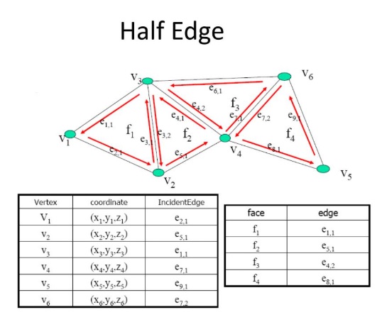
Boundary cells are special because the outer half-edge has no twin. This condition can be detected instantly at calculation time, and boundary cells can be treated differently. Boundaries are a big issue. The idea of a boundary is that it does something special to the data, for example in a fluid flow situation we can put a (non-porous) wall in place to create two fluid compartments, and along the middle of that wall the fluid velocity must be zero, because no fluid can get there. The enforcement of v=0 is an example of a boundary condition. There are many boundary conditions, walls can reflect or absorb, or absorb partially like in the case of an acoustic ceiling. In a neuron or an astrocyte, the plasma membrane is usually considered as a natural boundary, but there are many situations in which we'll have boundaries that are bigger or smaller than a single cell. In the volume conduction example we have an outer boundary which is the sphere, and inside a single neuron we have mitochondria and other organelles with their own membranes, which are also boundaries. So we have boundaries inside boundaries, we have a hierarchy of boundaries.

From a simulation standpoint, boundaries with fixed values are called Dirichlet conditions. There are other conditions, for example we can specify that the derivative at a boundary must be zero (instead of the value). Such weaker conditions are called Neumann conditions, after Carl Neumann (not John). There are also mixed conditions, and Robin conditions, and other forms. If a FEM simulation isn't working, it may have something to do with the boundary conditions. The finite element basis functions have to conform to the boundary. If the boundary has to be 0, then the basis functions have to be 0 there too. You may be asking yourself, how much of this we can actually see. The stalk of a dendritic spine is incredibly tiny, it's so small it's hard to visualize in a microscope. An astrocyte leaflet has about the same dimensions, it's incredibly small, so small it's hard to distinguish in a fluorescent image. We need a simulation to predict the things we can't see. With a traditional simulator we can see the synaptic activity, with a finite element simulator we can see the currents inside the spine, and with molecular dynamics we can even see the glutamate ions spilling over. But the finer the resolution, the harder it is to compute, and the more we have to place faith in the laws of physics.

Visualization is a big deal. There are plenty of programs what will let you visualize and manipulate a mesh, but when it comes to the display of fields on the mesh, we sometimes need powerful software. Visualization is computer graphics, and in that area there are many examples, from Hollywood and the animation world of gamers, to architecture and the modeling of stresses and strains in beams and buildings, to fluid dynamics as applied in weather modeling, to nuclear fission and fusion. Since simulations are so computationally demanding, we may be interested in reducing the visualizations to "only" the parts we're interested in. The good news is, that solid bodies are three dimensional, that's the most we ever have to deal with for computer graphics. Our simulation output comes in the form of "ticks", which are very much like "frames", they have a natural relationship with graphic displays. In the easy case, our task is reduced to mapping pixels, however in most cases we'll have to do some homogeneous transformations to get the visualizations we want.

When meshing, we'll need to visualize the mesh, and visualize the results on the mesh. Those are two entirely different things. To get a perfect mesh we'll sometimes need to edit it, and we'll certainly want to inspect it from every angle, so we really need a visualization tool like ParaView or Blender, and it has to be able to open files in our preferred format. However we frequently encounter meshes of a different kind, that are more structured than the typical Blender mesh. An example is a "structured cylinder" of the kind one might use to represent an axon membrane with embedded channels. Generally speaking, once we move from a surface mesh to a volumetric mesh, things get more complicated. First of all, very few tools can handle volume meshes. The best ones come from the fMRI world, where the machine generates voxels and those then have to be registered (aligned) with brain maps. Triangulating a surface mesh is not all that hard, but if we're mapping voxels on an astrocyte leaf with jaggy membranes we're going to end up with voxels that are only 1 nm on a side, because that is the resolution needed to overcome massive discretization errors at the boundaries. 3D tetrahedralization is difficult, the mesh needs to be pretty perfect to begin with, and the algorithms have to be told exactly what the constraints are, otherwise they'll fail.

There is a further issue that relates meshes and visualization. Think about the idea of placing organelles inside a neuron. To place an organelle that way, you have to "carve out" a piece of the interior volume of the neuron (in other words, you have to make space for the organelle). The organelle is a separate object, so there will be a boundary between it and the intracellular space, and the outer components can not cross that boundary. This is not like Blender or Maya where you can just place objects inside other objects without any constraints. In this case, biological objects are tied to the inner volume by specific scaffolding, via proteins that usually attach to the cytoskeleton. And the presence of an interior object requires a boundary at the level of the intracellular compartment too. A mitochondrion is a great case study because it's fairly large, and it has an outer membrane and an inner membrane, so it's a great exercise in boundary construction. Furthermore, the outer membrane of a mitochondrion has vastly different properties from the inner membrane or the plasma membrane of the cell, and the mitochondrion is frequently associated with endoplasmic reticulum which is yet another set of boundaries. If you're in the simulation business you're going to become an expert with boundary construction, it'll become like second nature to you. And it's a challenge, it's not always easy.

Much of the time, we need to visualize in detail what happens at the boundaries. This is certainly true in a nerve membrane, where we need to visualize the opening and closing of ion channels. We don't see the actual changes in channel conformation, even an MD simulation won't show us that, so what we have to do is estimate the opening and closing of channels in a small volume. And here's where the pedal hits the metal, because we need a relationship between the membrane voltage and the state of the channel, but now this equation is no longer represented as a friendly (if somewhat difficult) Hodgkin-Huxley equation, instead it's represented as a nasty stochastic differential equation with parameters we have to determine experimentally (because we don't really know what they mean). Instead of an Euler solver, we now have to use a Maruyana solver to deal with the statistical aspect of the result. The point being, we've left the simplistic world of NEURON far behind. Now we're in with the people who look at the air flows around the space shuttle when it's landing. We're solving stochastic differential equations on irregular geometry, that's what they do too. This is hard stuff, not easy to learn and implement. But at the end of the day, it makes the difference between the space shuttle landing safely or blowing up. There's a very famous story about the bolts on the Citibank building in NY - one morning the chief architect got a phone call saying the building would fall over in a high wind, and he said "no way, we did all the simulations", and in fact they had done so, but there was a single piece of paper, an engineering change order, that arrived "after" they'd done all the simulations, and somehow it slipped between the cracks and they ended up having to reinforce all the shock mounts in the building. The moral of this story is, the best simulator in the world isn't going to help if the rest of your process won't support it.

For serious high-power computational simulation, MOOSE is an option. MOOSE is a gigantic program that won't even install on most systems and doesn't have a Windows binary (use Docker!), but if you can get it to install, it'll do things for you that no other simulator can do. However, FEM in neuroscience is still a new concept, and therefore we're on the bleeding edge in terms of bringing our simple cable models into the real world. One must realize that porting a model to MOOSE (or even developing one there) is an enormous undertaking, and when all is said and done it's not even clear that we'll be able to visualize the results. MOOSE comes out of the supercomputer world, which has its own ecosystem and makes its own assumptions about the kinds of tools and support that are available. VTK is the most popular visualization tool in the supercomputer world, and it works there, better than it works on a PC. It's very easy to make VTK crash on a PC. I'm porting a supercomputer program to the GPU right now, and I can tell you, it's no fun. In a Python environment, there's a package called PyVista that you'll probably want to investigate if you're thinking about VTK or anything similar. PyVista is great, you can wrap just about any object and display it in a PyVista window, and in combination with other tools like Panel you can display it in a window inside a browser application. PyVista doesn't crash, but VTK does, so gradually over time you end up converting your VTK objects to native PyVista. And this is also a convenient point to port the display over to the GPU. When you get this environment running, you'll quickly realize that you're displaying things four different ways. Sometimes you need a server display, sometimes you need a workstation display, and sometimes you need a GPU display. Sometimes they all have to update at the same time. So the idea of a "simple dashboard" for this task, is a pipe dream. At minimum you'll end up with a user interface of approximately the same complexity as Blender. And at this point you'll have a choice: you can either try to package everything into one big gigantic end-to-end application, or you can try to break up your workflow into individual toolsets that can be re-used for different purposes. I'll remain agnostic as to which way is better, each way has its upsides and downsides. Personally I like the idea of small independent tools, because my experience has been that the big complicated ones are usually buggy. A small tool that does one thing exceedingly well is much better than a big tool that does everything for everyone but breaks all the time, in my opinion. Breakage causes frustration, and as a scientist I don't like frustration, we shouldn't have to jump through hoops to accomplish a simple task. (I say that with hoof firmly planted in mouth! :).