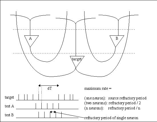
In an architecture where spike times are important, one can ask oneself “what is the smallest interval of time that can be resolved by a neural network?” If one imagines a neuron firing at maximum rate, the spike times are determined by the refractory period. If we imagine “all” neurons firing at maximum rate, we can stagger the spikes so they occur “dt” apart, and the resulting resolution is then approximately the refractory period divided by the number of neurons. In a human brain where the refractory period is about 1 msec and there are about 20 billion cortical neurons, this turns out to be a tiny fraction (about .05) of a picosecond.

If we instead use the prevailing estimate of 200 million processing columns ("minicolumns") in the cerebral cortex, the best case resolution reduces to about 5 picoseconds. Using an estimate of 2 million hypercolumns would give us around 0.5 nanoseconds. All these times, while fast, are physically realizable. The synapses don't work quite that fast, but in a moment we'll see how we can recover high resolution from a collection of low resolution components.

If we stipulate that neural updates are asynchronous, we can calculate approximately how many neurons can fire at once under these conditions (or let's say, within the refractory period of a single neuron, or any chosen interval in physical time). With no perturbance, we can use a Poisson model to estimate the intervals between spikes. Interestingly enough, a human brain is about 15 cm long from front to back, so at maximum velocity (best case, the speed of light, not accounting for wave propagation in an anisotropic medium) it takes a fraction of a nanosecond for an EM signal to get from one end of the brain to the other.

Relative to the concept of "dt", asking about resolution is the same as asking how quickly we have to update the neurons. In the original Hopfield network for instance, the asynchronous update mechanism is mandatory (the network won't work at all without it). The Monte Carlo selection of "the next neuron to be updated" ensures that only one neuron at a time changes state. (In reality this could be "one or a few" without disrupting the network dynamics, but at some point there is an upper limit beyond which the gradient descent mechanism will become confused).

Classic Delay Lines

To see how it's possible to get microsecond precision from a population of neurons that only fire milliseconds apart, we can look at a couple of classic examples from the literature, like the auditory systems of owls and bats, and the architecture of the cerebellum.

Let's say that a neuron (call it A) has an axon that's 10 cm long with a conduction velocity of 1 m/sec, and it's firing at a rate of 100 Hz. It will take each spike .01 second to travel the length of the axon. We can position another neuron (call it B) oriented in the opposite direction, so its axon overlaps that of A but the signal travels the other way. We can position neurons along the entire extent of these axons, receiving synapses from them, and these neurons can have a high threshold, so it takes both axons to be active at once to make them fire. Thus the neuron that fires will be at the location where the two signals meet. The figure shows this architecture applied to sound localization in the auditory system of the barn owl.

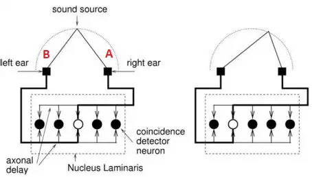
The time to space mapping is used by owls and bats to localize prey. The spatial map created from the two ears can be overlaid with visual maps from the eyes, and maps of head and body position. This helps the organism orient to the target even when it's moving.

Bats can individuate binaural signals with microsecond precision. The actual precision available in this design is determined by the number of neurons placed along the delay line, and the number of synapses into the delay line. If we place 1000 neurons along the delay line the .01 second resolution can become 10 microseconds.

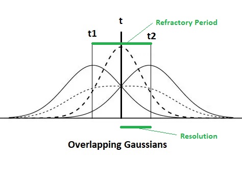
The ability to precisely discriminate time is enabled by the Gaussian shape of the connections between the delay line and the output neurons. This geometry is primarily determined by the shape of the dendritic trees of the output neurons. A sum-of-Gaussians operations helps to precisely localize the peak within the population. It is intuitive that in this kind of arrangement, there should be more neurons signaling actual time, than there are sampling points along the timeline. The architecture is such that there are never any "abruptly changing signals" from one moment to the next, once a nerve impulse has entered the timeline it never suddenly disappears, the axon never fails to conduct and never generates any spurious impulses. The figure shows a simple timeline that will give us 10 times better resolution than the refractory period of the individual neurons. In this network each output neuron represents a specific location in space, the one that fires determines where the sound is.

A different kind of delay line mapping occurs in the cerebellum, for a different purpose. The cerebellum is an integrator, its specific purpose is to time the input signals (which are mostly velocity-related) to the unfolding motor behaviors, and precisely tune the resulting limb positions to the desired ones. A considerable portion of the cerebellum is devoted to the oculomotor system, and we'll take a careful look at that particular function shortly. Generally though, the architecture of the cerebellum is consistent throughout, it does the same thing to all the circuits it participates in.

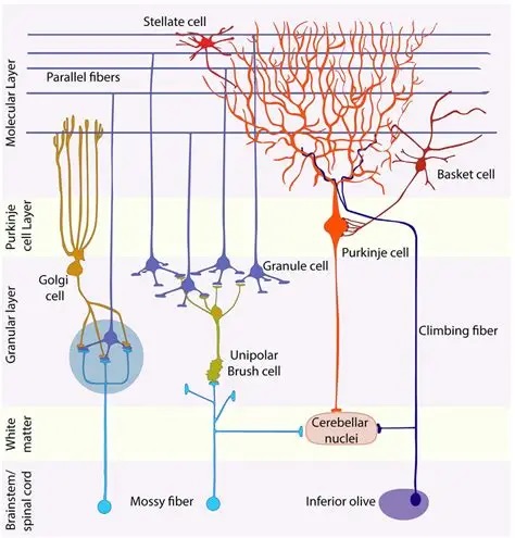
The input mossy fibers (which are excitatory) synapse in an intricate way with the dendrites of granule cells, the axons of which then climb to the cerebellar surface and branch into an oriented dipole about 3mm on each side. All of the granule cell axons are oriented the same way, and the dendrites of the Purkinje cells are oriented transversely so they connect with many granule cells. If we look at the synapses between the granule cells and the Purkinje cells, the convenient result is a synaptic matrix W, that relates granule cell activity G to Purkinje cell activity P.

P(i) = f ( Σ_j (G(j) * W(i,j) )

Equations of this kind are ubiquitous in neural modeling. In this case i represents the i-th Purkinje cell, and we are summing over all its inputs j from the granule cells. We multiply each entry by its corresponding weight in the synaptic matrix, and add them all to get an integrated sum that represents the total excitation to P(i). Then we take that result and run it through the threshold function f, which is typically an S-shaped (sigmoidal) curve like this:

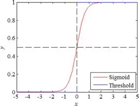
Of course this equation represents a "moment in time", because the inputs are constantly changing. Furthermore, with this approach we have completely ignored the time constants of neural and synaptic activity. Keep in mind that most forms of information transmission in the brain look somewhat like this, where the information from a point in time is spread out over a region of the timeline.

Even though synaptic matrices are very useful computationally, the picture of linear integration along dendrites is far too simplistic from a biological standpoint. Purkinje cells are multistable, they have multiple subthreshold stable states and their dendrites also generate small action potentials ("dendritic mini-spikes"), and these program the spike output in some highly nonlinear ways. We will return to look at the cerebellum in considerable detail when we talk about eye movements and the oculomotor system. For now the figure is meant to show the regular architecture and the topographic organization of some internal delay networks.

Network States and Phase Velocity

A neuron's decision "when" to fire is made stochastically on the basis of the state of the membrane. The membrane state is in turn affected by inputs and previous states. In a population of neurons, some fraction of them may be firing at any given time. In spiking networks or networks in which spike time is important, the stochastic behavior of the underlying ion channels can give rise to new dynamics that substantially influence the behavior of individual neurons.

When neurons fire at the same time, the synchronous activity can be recorded with multiple electrodes, and it can sometimes be detected from outside the cell in the form of "coherence" in the field potentials. Some networks have resonances, as do some neurons. One must be careful when studying models, to understand implicit sources of influence. At this point we can introduce the Nobel Prize-winning Hopfield model, which is a very simple omniconnected network with binary threshold neurons.

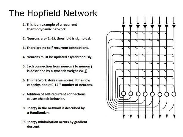
In this network, each neuron is updated independently. The "decision when to fire" is constrained by the design. In the model's original form, only one neuron at a time was updated, thus the network was "fully asynchronous". In such a network we won't see correlation between firing times, unless the window of analysis is very long. In real life, it's permissible to update "one or a few" neurons at a time, but because of the artifacts introduced by digital computer simulation it's not desirable to update all the neurons at once. Nevertheless there are many uses for synchronous updates, in various types of computations. This particular network, the Hopfield network, is very good at combinatorial optimization, but it takes too long for computer vision. Computer vision might be more amenable to synchronous processing, frame by frame.

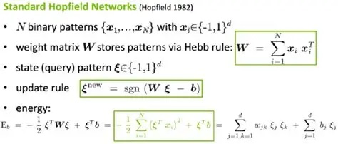
Another important concept introduced by the Hopfield machine is the "state" of the network. Since the neurons are binary, the network has 2ⁿ possible states, where n is the number of neurons. This approach is the basis for the statistical mechanical (thermodynamic) view of neural networks, which we'll develop on future pages. Whenever a bit (a neuron) is flipped, it changes the network state along with it. The magic of the Hopfield machine, is that the network state is related to a Hamiltonian (an "energy function") that depends on the configuration of bits (neurons) in the configuration space. In this way the state of the network is directly related to the state of its constituent neurons.

In Hopfield networks, the Hamiltonian energy function is debatably non-biological. These networks arose from physical analysis of the behavior of ferromagnetic materials, they didn't originate in neuroscience. Nevertheless, the need for an energy function and its computational usefulness encourages us to look for ways in which this functionality might be accomplished in real neural networks. For example, one could have a "master neuron" whose sole purpose is to average the population activity and feed the result back to the individual computational neurons. (There is little to no evidence for such a thing in real brains, except in very primitive organisms). Another idea is that the extracellular space somehow represents an "average" of neural activity insofar as its ionic concentrations change in relation to neural firing. (However this would require time for molecules to diffuse within a nucleus full of tightly packed neurons, and again there is no evidence for such a thing within the required time frame). Yet another idea is that this function could be carried out by astrocytes, which have all or most of the required connectivity, but in this case the Hamiltonians would be "regional", involving at most 100,000 neurons or so. There are other ways this can be accomplished too, but for the time being the existence of a neural energy function that is available for computations is still a matter of intense research.

It is worth re-emphasizing, that this network doesn't work at all unless the updates are independent and asynchronous. This network therefore operates quite differently from the back-propagation paradigm in machine learning. From a machine learning point of view, the Hopfield machine would be a form of "recurrent neural network" (RNN), since it connects with itself (that is, the outputs feed back to the inputs). But in a machine learning context, updating one neuron at a time would take forever, and performance is one of the major commercial drivers for artificial neural network technology. Nevertheless there are mathematical problems that combinatorial networks can solve very quickly, much faster than digital computers can (because of the parallelism). In the Hopfield network, the rate limiting factor is how quickly the neurons can be updated. The optimization works by "gradient descent" to minimize the energy function, and it can run until the energy stops changing (at which point it's reached a stable minimum).

In the original form of the Hopfield network, as shown above, there were no connections from a neuron to itself. If we introduce such connections, the network acquires new behavior, including chaotic dynamics. To the extent that such dynamics can be controlled, they can be computationally useful.

Let us engage in another thought experiment to understand the physical meaning of a picosecond resolution along the timeline. Let's say we have two neurons at opposite ends of the brain, maybe 15 cm apart, and neuron A wants to change neuron B's state. To accomplish this, two things are needed: first create the network state such that neuron B's bit flips, and then ensure that neuron B is the next one to be updated. Each of these actions has a delay (or "processing time") associated with it.

The first condition "can" in certain cases be met automatically when neuron A actually spikes. The physical processes that transmit the spike do not enter into play, only the network state. The network state is determined by a Hamiltonian related to the total energy, and this could be calculated by many means other than synaptic. (Gap junctions come to mind, for example, as does the extracellular milieu itself, and of course volume conduction directly related to electromagnetic transmission). In a real brain a neuron's transition to the unstable (spiking) mode might take a few microseconds (long enough for some ion channels to open up), but in a computer simulation a bit-flip occurs in less than a nanosecond, and this is how long it takes the network to change state.

The second condition can be met in a number of ways. The slowest way is for neuron A to signal neuron B using its axon, which has a typical conduction velocity around 1 m/sec. A much faster way is for neuron A to emit an electromagnetic pulse that crosses the brain at the speed of light, arriving at neuron B about 1/3 of a nanosecond later. In theory, if neuron B is in a critical or near-critical state at that point, the signal can directly and instantaneously affect the decision to fire. However, consider - does it matter "how" or even "why" the bit flip occurs, as long as it occurs? Let's say it occurs randomly. In this case, the information has been transmitted "virtually", and any subsequent measurement will verify that the information has in fact been transmitted. Can a neural network actually tell, whether the bit flip occurred randomly or whether it occurred causally?

Predictive processes that are able to control the stochastic behavior of neurons, can in theory support "virtual" exchanges of information. In every case, the fundamental unit of time is the duration, the interval. When the interval shrinks to zero, we get a peculiar form of "phase velocity", where signals appear to be propagated faster than they really are, with non-zero probability. What does this mean? For the sake of discussion let's be realistic and assume that only the cortical minicolumns form the timeline, and its resolution is in the picosecond range. A heads-up is, that even under these conditions, the network state will be updated a thousand times before an electromagnetic signal can get from A to B.

Where Is The Origin?

Again we're faced with the question of defining "now". The requirement is that a human brain be able to stage precisely timed behavior, either on demand or in response to environmental conditions. The human environment is constantly changing, it's very different from a machine learning experiment in which static frames are presented one at a time. One could dovetail these views using a sampling paradigm, but it's well known there is no clock in the brain and sampling occurs asynchronously (although in some cases it can be guided by population activity, for example thalamocortical visual signals are suppressed while eye movements are occurring).

Our concept of T=0 is much like the "seed" in fMRI studies, where one must choose a voxel as a base point. When we measure, "now" is wherever we put the electrode, and if we have an array of electrodes, we are measuring an array of "nows". The point being, they are not necessarily all the same. Even though they occur at the same physical time, the information in the representation space may be considerably different. Therefore correlations between the "nows" are the same thing as rotating our compactified circle, and doing some quick matrix multiplication at each rotation point. (If we had not compactified, this operation could be performed more laboriously with convolutions, although we would have to be careful at the boundaries).

Now we'll see how a neural network can make use of this information, quickly, efficiently, and seamlessly. Interesting things happen when we embed the compactified timeline into a larger network with more neurons and better resolution. To a certain extent, the compactified architecture will cause us to consider models of time "other than" the strictly linear physical model, even though physics is always physics and the laws of physics are the same everywhere. In a compactified neural network based on a loop topology, "now" isn't just a point in time, it occurs in a somewhat fuzzy manner within a window, in which neurons are being updated asynchronously even when their ultimate behavioral targets are all focused at a "point in time".