The brain is a window moving through time. The purpose of the brain is to optimize the behavior of organisms in real time, or as close to real time as is biologically possible. Real time implies the limit as dt => 0. In this section the structure and electrical activity of the brain are organized in relation to time.

Thanks in part to machine learning efforts, we've learned that spike times are important. We need to know "when" something happened. Matrix multiplication is not enough, and rate codes are not enough. The phase encoding of information in the hippocampus is proof enough of this assertion.

The Timeline of Electrical Activity

The brain is a window of neural processing, moving through time. Scientists frequently map brain electrical activity onto a “time line” defined by an imaginary clock, which is assumed to align with physical time. In experiments, brain activity is frequently mapped relative to the occurence of an event. For convenience, we can consider the event as occurring "now", and we can look at brain activity that precedes it and follows it.

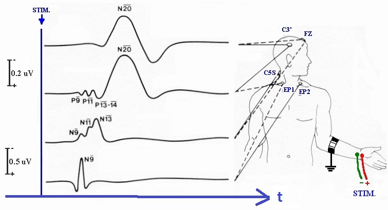
Here for example, is a series of evoked potentials recorded after somatic stimulation. The electrical activity can be traced through the brain, from one processing stage to the next, and you can see the peaks and troughs of the signals and calculate their delays from the point of stimulation. Each electrode provides a time series of voltage, relative to the time of the stimulation.

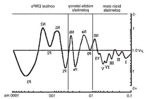
Here is the same thing for the auditory system, which has many identifiable markers, and the brainstem auditory evoked response (BAER) is an important diagnostic tool. A similar sequence of evoked potentials exists in the visual system, and we'll look at it in detail on subsequent pages.

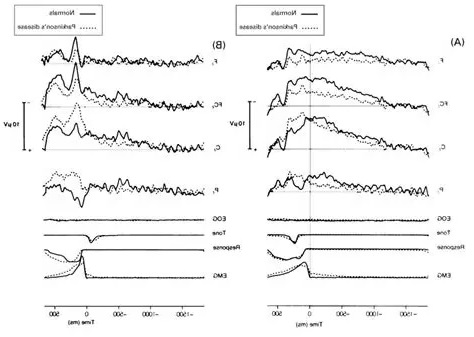
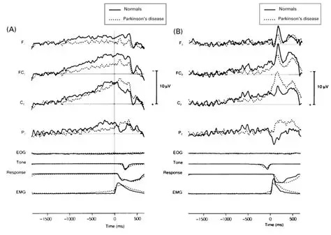
And here is a similar view of premotor potentials. Premotor potentials occur before a movement. In the figure below, the readiness potential in Parkinson's patients is compared to normal. You can clearly see that the electrical activity continues through the actual expression of movement. The movement is measured by the electromyogram (EMG), which is shown aligned with the time of the muscular event.

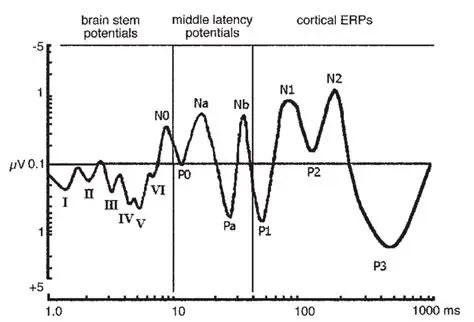
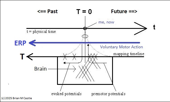
Evoked potentials occur after an event, and premotor potentials occur before an event. Combining and unifying these into a single map we can create a "time line" centered on the point "now", which we'll call t=0 (since it occurs "now" in physical time). And, we will explicitly map physical time into a representation space that is defined by the inherent architecture of the brain's neural networks. To distinguish the representation space from physical time, we'll call the representation big T, as distinct from physical time which is little t. This arrangement is shown in the figure. Here, the brain is a window moving through physical time, and note that the representation space T has the opposite orientation from physical time t. This is because T uses an egocentric reference frame, whereas t uses an allocentric reference frame. To align these two reference frames, we define "now" as t=T=0.

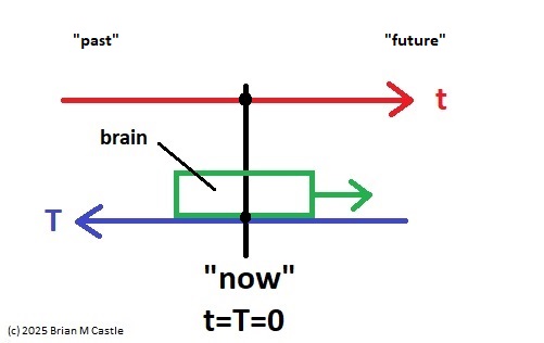
To get this orientation, we first flip the direction of the electrical signals, so the future is on the right and the past is on the left, like this:

Then we simply align the times of the event, and designate this point as "now", and represent it as occurring at T=0 in our mapping timeline. This way, the event related electrical signals move from future to past, just like they do in a real brain. The reason we do it this way, is to get the mapping to look like an ordinary time series, in the form x(t). This form of the signal is important because it generates a unified view in terms of predictions and outcomes, which will be useful for us in subsequent modeling.

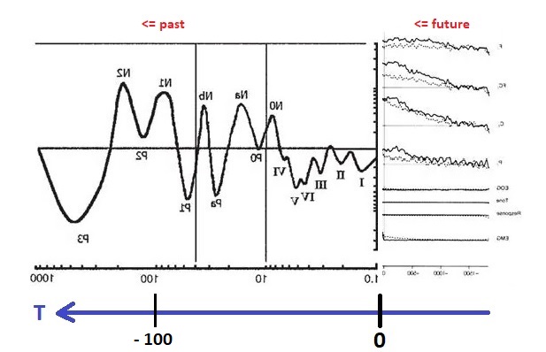
We must emphasize again, that there are two different reference frames involved in this mapping. T is "inverted" because of the way we just flipped the signals around. If one were to take a snapshot of the timeline at a point in physical time (say, t=0), one would see that the signal at T=-100 msec corresponds to an event that happened 100 msec ago.

In the above diagram, event related mapping occurs within the window shown in green, which advances along with physical time. However information relative to the point "now" moves in the opposite direction. Premotor potentials begin in the "future", and event related potentials map "past" environmental activity. T is oriented so it aligns with the time course of event related potentials. ERP's move in the same direction as T. T and t move in opposite directions (a time of T=-1 in the past means that physical time has already advanced to t=+1). T moves from future to past.

In evoked potential studies, "now" coincides with the presentation of the stimulus, and in premotor potentials it coincides with the effector action. Of course everything happens "now", in real physical time. However the information attached to these events is disseminated in different ways along the timeline. In the simplest case we have an electrical signal we can measure, and the waveform usually shows a peak or trough at a characteristic delay in relation to the stimulus.

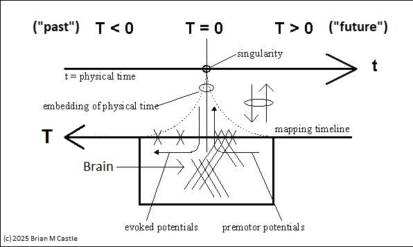
The figures show such a timeline defined by brain electrical activity. Little t means physical time, and big T is its representation in the neural network. The figures show a mapping between the two. The area labeled "Brain" will be discussed in detail, for now it can be loosely considered as the brain's processing window. The figure shows an unfolding of physical time into the representation space, which is an important element of the timeline model related to its topology.

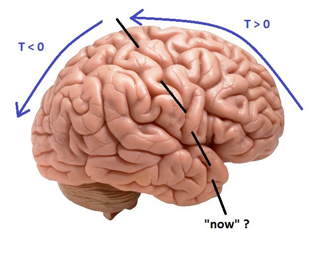
Using this model, we can see that the activity related to a voluntary motor action travels in the direction of the blue arrows, it begins on the far right at T > 0 (“future”), travels leftward through the singularity at T=0 (“now”), and finally the sensory consequences appear on the left side at T < 0 (“past”). Such a mapping dovetails with perceptual experience insofar as time often seems to flow “through” us, from future to past.

Loosely speaking, at a very high level, the human experience of time maps onto the circuits of the brain. We say we look "forward" to meeting you, and we look fondly "back" at all the good times we had together. This arrangement is conceptualized in the figure, and dovetails with the idea that voluntary motor activity begins in the front of the brain and sensory information is processed in the back (and sides, the division being most prominent at the level of the central sulcus).

What Is "Now"?

The brain's idea of "now" turns out to be considerably different from the simplistic idea of time locking to physical events. We will develop the concept of "now" piece by piece on these pages. Our brains take "now" apart, and put it back together again, in a different way that's more suitable for information storage and recall. Much has been made of the grid cells in the brain's entorhinal cortex, and their cousins the time cells. The exact nature of the conversion between egocentric and allocentric reference frames is not yet known, but we do know it occurs, and it likely involves neurodynamics since it seems to be closely related to theta wave oscillations.

Humans can estimate durations at much longer time scales than the extent of detectable ERPs in the brain. One of the important areas for current research is how the synaptic events that occur on msec time scales come to influence neuronal behaviors in the seconds to minutes range. We can estimate time on longer scales too, however these estimates are increasingly variable with delay and often depend on the state of the individual. The mechanism for estimating duration is not yet known. Ramp activity in the entorhinal cortex does not necessarily indicate duration, more likely it simply encodes the sequence of events. Time is only explicitly mapped within the window defined by the boundaries of (detectable) event related activity.

One can argue about where those boundaries are. In humans there is detectable event-locked electrical activity a second or more away from T=0, and the time course of short term plasticity may be on the order of seconds to minutes while the time course of long term plasticity may be on the order of minutes to hours. Conceptually however, these things are different from the highly nonlinear and stimulus-evoked associative functions that recall information regardless of its point of origin. The latter representations are, effectively, timeless - and how they get that way is an open question, which we'll look at in the upcoming pages.

Why Machines Are Different

In a nutshell, "artificial" neural networks are different because they have little to no dynamics. As close as machines come to dynamics these days is Poisson modeling of spike rates. The figure shows a feed forward path mapped onto a layered neural network architecture, and the information flow associated with a voluntary motor signal (oriented the same way as the related ERPs). There are some noteworthy differences between this figure and the neural timeline. Can you spot them?

In the above diagram, if this were a convolutional machine network, the retina would be on the right and the inferotemporal cortex would be on the left - but notice, there is no oculomotor system. There is no concept whatsoever of an optimization related to the current moment. In a typical machine learning paradigm, the error signals related to synaptic updates are transmitted from layer to layer all at once, by backpropagation. This is highly non-biological and directly contradicts the requirement that neural updates be asynchronous (which we'll discuss in detail shortly). There is an explicit representation of time in such networks, in the form of "ticks" during which the calculations occur. The network's understanding of time is the computer clock that relentlessly sweeps back and forth, transmitting information from one end to the other in an immutable cycle.

Whereas, biological systems are highly dynamic. There is no clock in the brain, instead there are measurable oscillations at all levels of resolution, ranging from milliseconds to days. Sometimes they're coherent, and other times they're wildly incoherent and chaotic. Brain waves are an important but tiny part of the picture. For example subthreshold oscillations of the membrane potential in individual neurons are related to the inter-spike intervals in the burst that occurs after inhibition. Dynamics are difficult to capture in computer simulations. The market for AI is driven by response time, so a lot of attention has been paid to performance driven architectures that can make use of nVidia GPUs for matrix multiplications. However it would be very difficult to solve 100 billion simultaneous differential equations in real time, even with massively parallel computers. Actual devices are needed, perhaps memristors or photonics or something similar.

The predictive coding paradigm partially avoids this issue by allowing neural updates to occur asynchronously, so there is no "back propagation" per se, although the calculations are still computationally expensive. Nevertheless the model is not in the business of creating brain waves, and it doesn't use any kind of phase encoding (although that could be introduced). The combination of predictive coding with neurodynamics is a powerful tool, allowing large amounts of concise information to be transferred in short periods of time. One of the main reasons for using artificial network models is to be able to study behaviors like "chaos", and this is difficult with backpropagation architectures, however it is mathematically accessible with a predictive coding network endowed with an embedded timeline architecture. (It isn't "easy" that way, but the tools do exist, and many mathematicians and engineers are already familiar with them, and some biologists are too).

Conversions between timeline orientations can be made quite conveniently by considering T = f(t). In our chosen representation in the diagram, the future is on the right (T > 0) and the past is on the left (T < 0). From an egocentric vantage point, signals move from future to past (or from now to past, in the case of a sensory signal). Voluntary motor actions enter the timeline at the far right, and travel leftwards. So do predictions, and anything else that needs to be accessed at T=0. Sensory events enter the timeline at T=0, and move leftwards. Some of them represent the consequences of actions, some of them represent materialized predictions, and others are simply sensory events from the environment.

The boundaries of the timeline are significant. After an evoked potential reaches the left end of the timeline, what happens to it? In a human brain, sensory events enter the hippocampus where they are transferred to short term memory, and important events eventually get consolidated into long term memory. Evidently, memory is both the destination of all information, and the source of all information, insofar as stochastic behavior emitted by a network is weighted by transmission through the synapses.

For a heads-up on some of the concepts that keep this view tightly tied to physics and biophysics, check out this article by Karl Friston that talks about the free energy principle. Box 2 shows the incredibly simple neural network that supports it, and Figure 4 shows many of the things it applies to.