The idea of a neural "timeline" is useful in many ways. To understand some of the possibilities, we can use the timeline like a retina, and imagine we have an observer that can see the entire pattern of activity along the timeline at once. Such sampling can occur either synchronously or asynchronously, or somewhere in between (for example phase locked to a local alpha rhythm). The observer doesn't have to be centered at T=0, it could be anywhere, and it could see the whole time line or just a portion of it. (This concept was shown on the previous two pages).

It is perhaps easiest to consider the power of a mapping timeline in a machine learning context. With the usual Hebbian and nearly-Hebbian learning rules, a neural network will come to respond to the statistics of its input. In a visual system, that will be the statistics of the images on the retina, and in a mapping timeline with well defined anchor points, such statistics will include the intervals in the neural dynamics (like the distance between the N70 and N100 in the visual evoked potential shown earlier). So a hypothetical observer that sees the entire timeline as a retina (a "snapshot" of a collection of time series) will be able to track a voluntary motor movement as it elaborates along the timeline, including ultimately its sensory consequences. This is how the consequences of voluntary motor actions are separated from simple sensory input - the brain predicts the sensory consequences of an intended motor action, and then tracks it along the timeline as it elaborates. To do this, it has to understand the joint statistical distributions between the predictions and the outcomes. Thus a "covering" comes to mean more than just an extrapolation through the blind spot. It is, in fact, a topological embedding.

The architecture of such a covering is as simple as feeding one network into another. The usual way of doing this involves a synaptic matrix, but it can be done in other ways too. For one, we can actually physically embed one network into the other, complete with local and global co-wiring, so that multiple synaptic matrices as well as gap junctions and the intercellular milieu come into play. This is probably a more realistic model than the simple diagram below, but the diagram illustrates the main concept. We're going to embed the compactified timeline into another network, that entirely covers the connection space at a fine level of resolution.

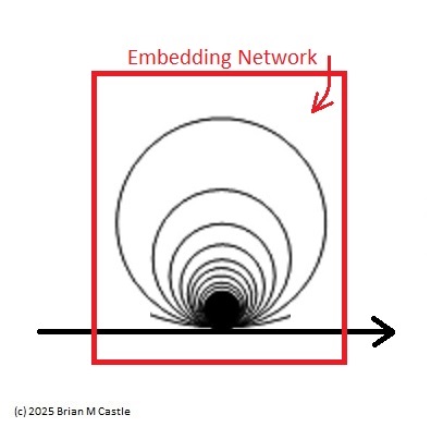
The concept of a topological embedding is somewhat complex, and we'll develop it piece-wise in the coming pages. Fundamentally it's exactly what it sounds like - a mapping. A point mapped into R¹ is an embedding, and a line mapped into R² is an embedding, and a compactified line (a circle, as shown in the above figure) mapped into a plane in R² is also an embedding. In this instance, it's a mapping into a higher dimension - essentially from R¹ to R² except we've "extended" R¹ prior to the mapping by compactifying it.

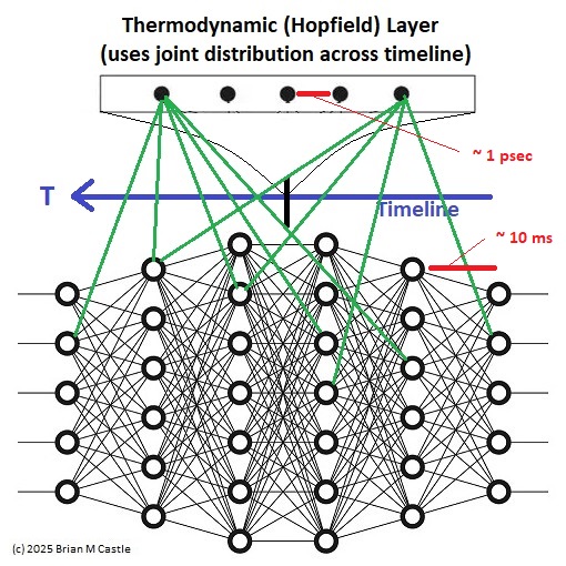
In terms of a neural architecture, an embedding can be considered as a mapping between dimensions. Some representative architectural candidates exist in the cerebellum and the hippocampus, as well as in the cerebral cortex. A neural embedding is much more than just an overlay though, and it depends heavily on the underlying connectivity. It can't be fully shown till we have a detailed understanding of network architecture, so... hang in there! Till then, we'll consider it loosely in terms of two neural systems occupying the same synaptic space. One such arrangement is shown in the figure. In this diagram, the transmission time along the timeline is much greater than the bit-flipping time in the Hopfield ("thermodynamic") layer. The result is that the Hopfield layer learns the "trajectories" through the timeline. (The word "thermodynamic" in this case is used loosely to indicate a network that depends on an energy function).

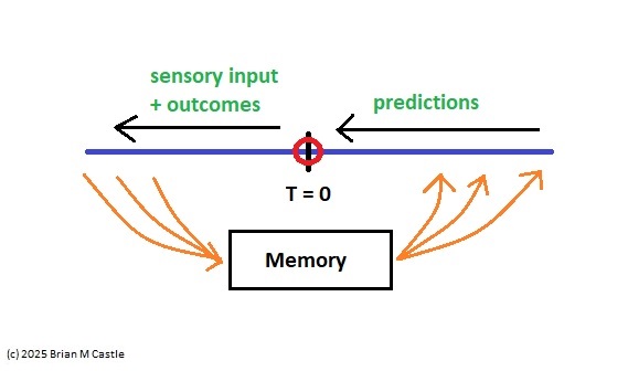
The singularity at T=0 has a counterpart at T=∞. It is important that this point be topologically compact, so information can flow "through" it (for one thing, we need to calculate derivatives at this point, otherwise we'll be unable to assess the accuracy of our predictions). The point at infinity represents memory, in the limit as dT=>0. This is where sensory information becomes prediction. Note again, that in the earring topology, all the points at infinity line up. These are effectively "models" of the point T=0, at different time scales.

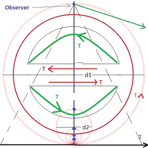
In doing this, from a control systems standpoint, we're turning each timeline interval into a Kalman filter with a time constant approximately equal to the window width. The Kalman filter is intimately related to the Bayesian filter, at some point the two become one and the same. We are predicting the network activity in the neighborhood of T=0, from the vantage point of the compactified points at infinity (the distance between these points and the linear origin "now" represents the inherent delays of transmission through the filter). While the timeline is directional on the basis of genetically programmed brain wiring, the embedding network is inherently non-directional. When this network organizes itself, it will be driven by the causal character of events in the environment. The flow of time in the representation space will be from future to past, and the same orientation will apply to the induced internal events. This provides us with an immediate link to the "directed acyclic graphs" that are so important in causal analysis and causal modeling (meaning, the elaboration of motor behavior).

From a machine learning standpoint, a proper embedding requires that we access both the original timeline and the compactified timeline. This allows us to "project back down" from a hoop to the line segment. However when we do this, something interesting happens to the orientations. If we place an observer at the point at infinity, looking straight down at T=0, and project the compactified view back down to one dimension, the information travels in the correct direction along the bottom half of the circle, but it travels in the opposite direction along the top half. This results in some interesting abilities relative to the determination of causality, and it also explains the "backwards replay" observations of the neural activity in areas like the prefrontal cortex and hippocampus.

Note also, that this architecture dovetails perfectly with the concept of phase encoding (as found in the hippocampus), since a compactified loop is periodic. In essence one can take a snapshot of the entire timeline including premotor and evoked predictions, and phase encode the whole thing into a single gigantic spike train (indicating "where" the activity occurred along the timeline, which means "when" in time).

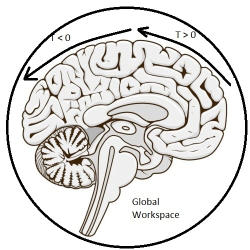
The Global Workspace

The timeline mapping of brain electrical activity ties together concepts as diverse as predictive coding, free energy, dynamics and criticality, information geometry, memory, and even the global workspace related to consciousness (Baars 2005). In these pages we'll talk about each of these topics, after showing a couple of examples of real sensory and motor systems in the brain.

The concept of the global workspace arose from the consideration of memory. Is there one large memory store, or are there many small stores? If there are many small stores, are they organized by function (like, visual information is stored in the visual areas)? If there is just one big store, it's pretty clear it'll have to be accessed in different ways. There is "working memory" that pertains mostly to real time sensory input, there is "short term memory" that relates to scene mapping and navigation, and there is "long term memory" from which we can pull information regardless of when it actually occurred (so in a sense, information is becoming more "time-independent" as it's being stored). If there is just one big memory store, clearly some kind of control system is required to organize all the different ways it needs to be accessed.

However here in this discussion, the global workspace takes on an expanded meaning. Not only is it intimately related to several kinds of memory, but it's also required computationally, and it hosts interesting, visible, and computationally useful behavior around its dynamics, which may include critical points, and controlled deviations from those points. In fact, it "embeds" the timeline. It handles the joint distributions of the motor predictions and the sensory consequences. With a little bit of architectural magic, it can even predict its own next state, at the same time it predicts trajectories through the timeline.

In a compactified architecture one can envision that each point in a loop is looking out at all the other points, creating its own “view” to the activity along the timeline. A wide variety of learning rules can be used to self organize these points. Some rules are entirely local at the synaptic level, some depend on the local extracellular milieu, some depend on astrocyte activity, some depend on a network Hamiltonian. We wish to self-organize in a manner that is suitable to the task at hand, so different portions of the network will need to self-organize in different ways at different times. However the embedding network will act to smooth regional development.

One of the very powerful aspects of this architecture is its leverage of the predictive capability. If we're being "neuroscience sticklers" and insisting that back-propagation is non-biological and shouldn't be used in our models, then we must use a predictive coding paradigm where errors are explicitly represented in the firing of neurons. This type of "real-time" activity is considerably different from the processes involved in memory consolidation, and many of these processes begin to make sense once it's understood that a translation is needed between memory and real time. Clearly, each point along the timeline needs access to memory (if it doesn't have it, it can't make the next prediction). In a timeline architecture, the timeline handles real time, and the embedding network handles the global store. The relationship between the two is of intense interest in current research.

A specific design point required by the timeline embedding is the coupling of the behavior along the timeline to the behavior of the embedding network. This coupling can occur in many ways (simultaneously), and there is overwhelming evidence that the brain uses all of these ways at various points in the design. The most obvious (and perhaps least interesting) coupling occurs at the synaptic level, when there are mutual connections between the two networks. In a real brain, coupling can also occur electrically and ephaptically, within the window defined by the timeline.
The width of the singularity around the current moment can be minimized in some intriguing ways. The timeline maps time to space, so it becomes very much like a retina, in the sense that an observer gifted with a topographic mapping will see a pattern of moving information with near-continuous estimation and prediction through the blind spot. Taken in its entirety, the pattern on the timeline at any given moment contains all of the "active" information that is being predicted and optimized relative to the next moment. This ability is enabled by a mapping of all the "trajectories" through the neighborhood of T=0. When these are statistical trajectories that can be described by distributions, the resulting manifold becomes computationally accessible.

What Is "Now"?

The base point of the representation in the embedding space is implicit, it's an affine space where the origin is only "somewhat" defined. We can reasonably determine its neighborhood, but we can't pin it down. It is... "uncertain". In a way it can even be said to "wobble", based on the inherently stochastic activity of all neural processes. What ties the network information to physical time is the flipping of a bit in the network (or equivalently, any other detectable physical event). The timeline information related to the distance between a state change and the bit flip that led to it, is what the earring architecture unfolds. (The activation of a muscle fiber in the periphery is a bit flip just like any other, since ultimately everything is part of the same network).

The takeaway from this overview is that "now" in our subjective experience isn't a point on the timeline, it's an active synthetic construct that depends on an unfolding of event-related activity into the embedding network. There is no point labeled "now" in the embedding network, the whole thing is "now". Except that "now" has somehow become a window, instead of a point in time. A topological unfolding maps the timeline into the embedding network. Consequently, the embedding network treats the pattern of activity along the timeline as an input that rapidly changes state. With respect to the update capabilities of a Hopfield network, the machine learning community informs us that certain extensions to the basic design are helpful for reliable and efficient sequence learning. These go by names like dense Hopfield networks (Krotov 2023), temporal kernels (Farooq 2025), generalized pseudo-inverse rules (Tolmachev & Manton 2020), temporally asymmetric synaptic modification (Aenugu & Huber 2021), and input-driven dynamics (Betteti et al 2025).

In a modeled form (which most likely very closely resembles a machine learning architecture), this embedding model requires asynchronous updates, it will not work with a synchronous network. Which is actually a good thing, because it forces us to be real. Synchronous backpropagation won't even work with this model, so there's no need to consider it further, except insofar as it may be useful for certain aspects of training, which we'll get into later in the section on plasticity. Asynchronous predictive coding is the best way to endow the embedding layer with the computational power needed to handle the timeline.

Based on the presentation so far, the timeline is capable of phase-encoding a spatially mapped time series into a spike train. This is important behavior that we'll return to again (several times!). But what about chaotic behavior? Chaotic behavior is important because it is deeply correlated with consciousness, as outlined neatly by Toker et al (2022). All these things tie together, at the level of predictive coding, inference, and causal navigation. Those may sound like big words, but they're quite manageable in the context of an appropriate model.

Above is an oversimplified depiction of the brain's neural circuits embedded into a larger network called the "global workspace". In reality brain wiring is very specific, for example there are small nuclei in the brainstem and thalamus that regulate important aspects of consciousness. Lesions in a tiny cholinergic cell group in the rostral pontine tegmentum result in coma. The regulation of consciousness is generally taken to be distinct from its content, and this separation pertains directly to neural network architecture. There are certainly areas in the brain that serve as "control systems" to regulate dynamics rather than data.

However the cerebral cortex is relatively consistent in its architecture, give or take. The six layered architecture is ubiquitous in the neocortex with very few exceptions. Some areas are more granular than others, and in some the layers can be more easily distinguished, but generally speaking the internal wiring of the neocortex and its columnar organization are pretty consistent. In a timeline embedding such as the simple one shown on these pages, it is important to realize that there are actually three networks in play all at once - the linear timeline, the compactified timeline, and the embedding space. Each cerebral column is connected into all three. The nature of the connection is only partially understood at this time, but it is becoming clear that each processing column has a predictive view to the signals that it processes.

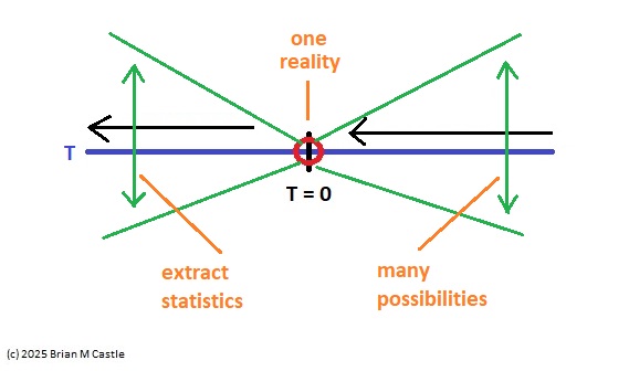
When we put all the individual views together, we arrive at a “universe of possibilities” generated by the various points in each timeline. These are predictions not directly tied to environmental events, they are "internal information" and yet they appear along the timeline just like environmental events. In this way the timeline ends up analyzing the embedding space too, and a topographic mapping of the timeline is sufficient for the embedding space to program the timeline. The individual views are asynchronous and we can surmise that the representation of time in the embedding space is therefore "fuzzy", it works on dynamics rather than topography. The views are kept in synchrony as needed, by neurodynamics, brain waves, gap junctions in neural and glial syncytia, and so on.

Once we have individual views from the compactified timeline, we can vectorize them and feed them into the embedding network, which will match events with expectations (since they're both part of the input), and to the extent an expectation can be tracked along the timeline, we can say the network is “aware of” its materialization. (We won't say "conscious" of, because that means something specific and it involves meta-processes including an elaborate control system).

In a sense the sum total of the predictive activity in a human brain is “faster than real time”, and that’s where awareness lives, it lives in the “dt” just ahead of t=0. The requirement is that there be “enough” neurons to achieve the needed resolution. Surprisingly, this number seems to be pretty small, preliminary calculations indicate it's in the 100 million range. Therefore some brains can not be conscious. Cats and dogs may qualify, but most insects and fish do not.

Probably some rudimentary form of awareness can be acheived with fewer neurons, but this is currently difficult to define and impossible to measure. However humans and many animals can report subjective experience, and the Libet experiments show clearly that the conscious process is something different from the actual timeline. In humans it takes about half a second for events to enter consciousness, and our brains fool us into thinking we’re aligned with real time!

The Window of Awareness

Our brains are windows moving through time. If one considers all possible delay-related activities, one would have to conclude that they are “large” windows, almost infinite. Delays that are longer than the extent of the timeline are stored in short term memory or long term memory, and motor behavior is the result of stochastic activity combined with memory, and these relationships would be impossible to tease apart with conventional methods (even Volterra-type noise analysis) because they’re data dependent (the assumption of stationarity is violated).

On the other hand, one of the consistent features of human experience is its continuity. In the subjective world, the flow of environmental events seems approximately continuous. Different time scales seem smoothly related to one another. However in brain architecture as we understand it so far, there are distinct clusters in the time constants associated with neural processes. Nothing is "continuous", in the sense of subjective experience. Molecular events occur on microsecond time scales, neural firing is in the millisecond range, and event-related electrical activity covers seconds. How is it that processes like memory and long-term planning can seem to be smoothly integrated at time scales that are much longer than any known neural processing?

Part of the answer comes from machine learning. Information at time scales longer than those supported by the computational network, can be evoked by data. The associative memory paradigm is timeless, it lives outside of the space of time-locked systems, except insofar as the processing delay associated with the time it takes to recall a memory. As already suggested, our brains have specialized architectures that integrate long-term information with short-term dynamics. The machine learning community has not yet fully explored these architectures, although it's rapidly covering the territory - but as neuroscientists we can look ahead and point out some of the obvious features that make this system work. We'll discuss scene mapping and short term memory in detail, and its relationship with phase encoding and information compression - but so far it seems intuitive that there is specialized processing that lives around the point at infinity, that somehow "extends" the timeline and makes it seem nearly infinite in our subjective experience.

While discussing the mathematics of phase encoding, it's worth keeping in mind that the human brain is wetware, it's stochastic, noisy, and chaotic. And neuroscientists have to tease apart wiring that's determined by genetic markers, it doesn't have the benefit of being neatly layed out on a PC board with CAD/CAM.

At this point in the discussion, we can look at the above figure and determine at a glance that the machine network is not compactified and doesn't have any idea of "now". And it's quite obvious that the biological network isn't quite as neatly organized as its machine counterpart, the layers are somewhat indistinct and there is all kinds of wiring that bypasses layers. However one can think about an extended timeline that's "not" compactified, and how exactly it would have to work to get information from memory into motor action. (Robots do this, but they have the benefit of a clock to synchronize the circuitry - and there is no such clock in the brain).

There are models that do not require an "infinite" timeline, and a bounded timeline gives us a convenient way of understanding the roles of brain structures like the hippocampus and the prefrontal cortex, that operate at T << 0 and T >> 0 respectively. There is considerable evidence for a "grid" of temporal relationships in the human brain, that operates very much like the range of spatial frequencies in the visual system. This mapping in humans lives in the area around the hippocampus, in the entorhinal cortex, perirhinal cortex, parahippocampal cortex, and internally to the hippocampus in the subiculum and the fields of the cornu ammonis. An open question is whether such structures map activity onto the timeline, or extend the timeline, or both.

There are also structures that straddle T=0, the claustrum is one of these. Electrical stimulation of the claustrum disrupts consciousness in humans, and sometimes creates subjective experiences. There are many other structures that straddle the midline, on the T=∞ side instead of the T=0 side. And these structures are often independently embedded into portions of the timeline according to local processing requirements. (For example area LIP in the parietal lobe processes 3-d spatial information and provides a spatial map to the frontal eye fields that guides voluntary eye movements, and both areas are directly connected into the brainstem oculomotor system at the level of the superior colliculus).

Considerations related to perceptual delays make some kind of timeline embedding mandatory in the brain. For example the Libet experiments show that the conscious process "binds" activity occuring now to activity that occurred half a second ago. Zeki (1975) points out that for brief stimulus exposures, humans perceive color about 40 msec before we perceive form, and about 80 msec before we perceive motion. These various delays need to be aligned to arrive at a uniform and continuous awareness.

The timeline model makes specific predictions that can be tested experimentally. It differs from machine learning models in that it engages dynamics, which the machines find difficult because of the performance factors involved in solving differential equations. However it is compatible with Bayesian inference and a host of other information generating methods that are useful and necessary in the real world.

One of the very interesting questions is the relationship between information and chaos. Neural networks are capable of various chaotic states that seem to have a very close relationship to consciousness. Do these states exist along the timeline, or are they a part of the embedding space, or how exactly do they work? To begin answering this question, we need to know a bit about neurons.